The 2D-QSAR wizard
The nine pages of the 2D-QSAR model builder: every option, its default, and when to change it.
Wizards > 2D-QSAR model builder collects the settings of one regression study and builds a workflow from them: read the data, curate the structures, compute descriptors, split the compounds, fit the model and validate it. When you press Build model on the last page the workflow opens on the canvas and runs, and its dashboards open when it finishes (see The model dashboard). Because the result is a workflow, every value the wizard chose can be inspected, changed and run again, and the same file runs unchanged from the command line.
The wizard has nine pages, listed on the left: Data, Curation, Descriptors, Preprocessing, Training and test sets, Descriptor selection, Model, Validation and Output. Next and Back move between them, and a page that has been completed shows a tick. Explanations are tooltips: rest the pointer on a label. Most pages end with More options, which lists every remaining parameter of the workflow node behind the page with the range and choices the node declares; a value set there overrides the page's own control. For classification models, see Classification models.
1. Data
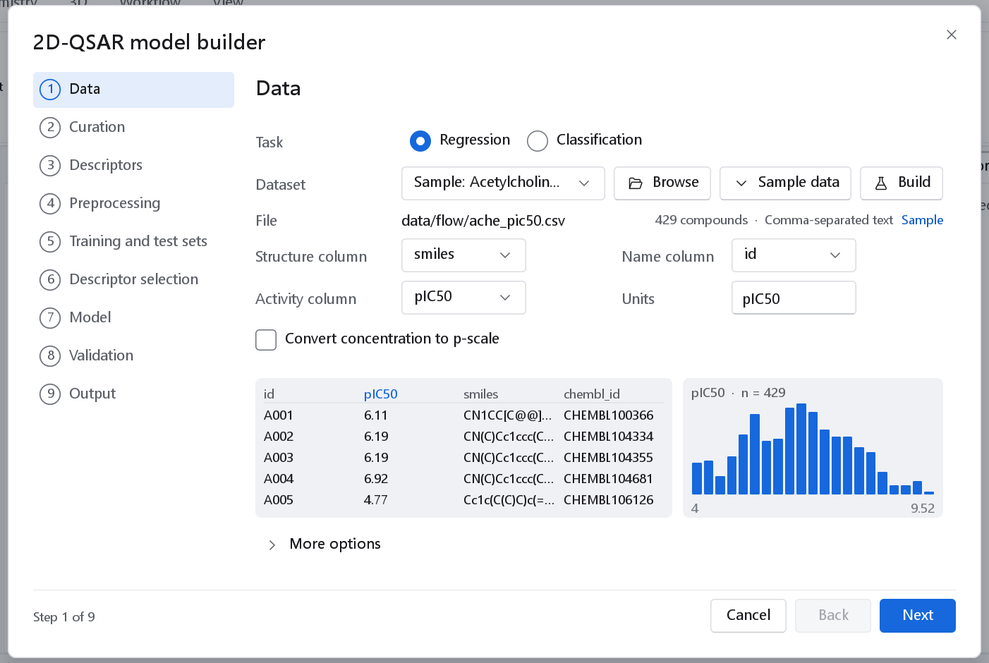
| Control | What it does | Default and when to change it |
|---|---|---|
| Task | Regression models a measured value, Classification a class label. Switching the task applies the default recipe of the new task; the data, the curation, the outputs and the More options values are kept. | Regression. |
| Dataset | The open datasets, or a file. A dataset that was edited since it was imported (rows removed, sets assigned, columns added) is written as a Snapshot and the workflow reads that, without excluded rows, rows without a structure, hidden columns or descriptor columns. | The dataset you are working with, or empty. |
| Browse | Any structure file or table: SD, MOL, MOL2, PDB, XYZ, SMILES, CSV, TSV. | |
| Sample data | The example data sets shipped with the program. | Used only when you pick one. |
| Build | Opens the Dataset Builder to assemble a dataset from ChEMBL, PubChem or files (see Building a dataset from ChEMBL). | |
| File | The file the workflow will read, the number of compounds and the format. | |
| Structure column, Name column | For tables: the columns that hold the SMILES and the identifier. The lists hold only the columns the file has. A column recognised from its header is pre-set and tagged Suggested until you confirm it. | Check the suggestion. |
| Activity column | The numeric column (or SD data field) to model. | Must be on a logarithmic scale for the usual acceptance criteria to make sense. |
| Units | Free text for the axes and the report. | |
| Convert concentration to p-scale | Adds a transform pX = -log10(X in mol/L), the "p" notation of the IUPAC Gold Book, with the unit the file uses (nM by default). Values of zero or below cannot be converted and are refused. | Off. Tick it for a column of IC50, Ki or EC50 concentrations. |
The page reads the file at once and refuses what cannot work before anything is computed: a column the file does not have, an activity column that is not numeric, or fewer than 10 compounds.
When a series is likely to be hard to predict
Once the activity column is set, the page measures two properties of the series: the standard deviation of the activities, and the density of activity cliffs, the pairs of compounds with an ECFP4 Tanimoto similarity of at least 0.8 whose activities differ by at least one log unit, divided by the number of compounds. When the standard deviation is below 0.75 log units, or there are more than 0.5 cliff pairs per compound, an amber note appears under the column choices, for example Note: activity SD 0.18 log units; such series were often hard to predict.
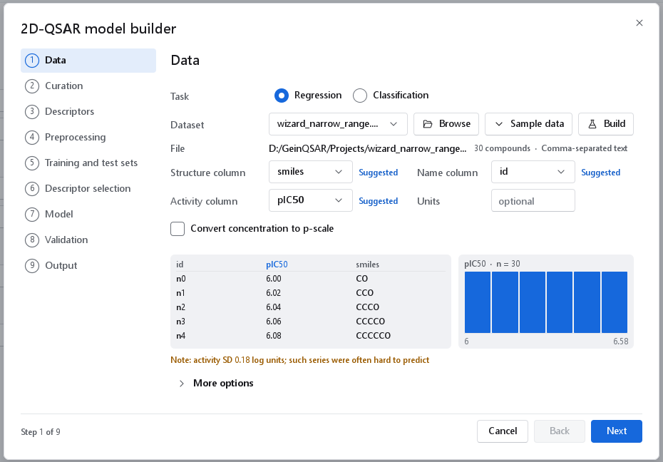
The tooltip states what was measured on your series, and what we measured on 90 independent ChEMBL series of 32 to 131 compounds: the default model predicted a held-out set better than the training mean on 12 of 20 series with an activity standard deviation below 0.75 log units, against 53 of 70 above it, and on 3 of 6 series with more than 0.5 cliff pairs per compound, against 62 of 84 below it. It cites Tropsha (Mol. Inf. 2010, 29, 476) for the limit a narrow activity range places on predictivity, and Maggiora (J. Chem. Inf. Model. 2006, 46, 1535) for what activity cliffs are.
2. Curation
Salts, counter-ions and charge states are not part of the structure-activity relationship but change every descriptor, so structures are standardised before anything else.
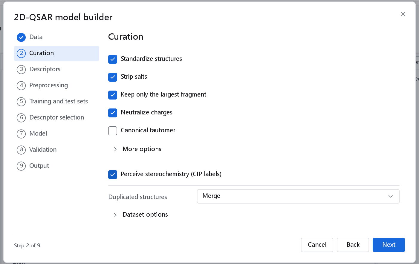
| Option | What it does | Default and when to change it |
|---|---|---|
| Standardize structures | Switches the four steps below and the options under More options on or off together. | On. Turn it off only for structures that were curated already in exactly the way you want. |
| Strip salts | Removes counter-ions and known salt components. | On. |
| Keep only the largest fragment | Keeps the largest connected component, for mixtures and solvates. | On. |
| Neutralize charges | Neutralises ionised acids and bases where a neutral form exists. | On. Turn it off when the charge state is the point (quaternary ammonium series, for example). |
| Canonical tautomer | Replaces each structure by one canonical tautomer, so that two tautomers drawn differently give the same descriptors. | Off. Tick it for sets drawn from several sources with inconsistent tautomers. |
| More options | Remove explicit hydrogens (on), Disconnect metals (on), Normalize functional groups (on), Remove isotope labels (off). | |
| Perceive stereochemistry (CIP labels) | Assigns R/S and E/Z labels. The chirality-aware descriptor families need them; without them two enantiomers are indistinguishable to the model. | On. |
| Duplicated structures | What happens to several rows of one compound, compared by canonical isomeric SMILES after standardisation. Merge: one row per structure, agreeing values averaged and contradictory groups removed (Fourches, Muratov and Tropsha, J. Chem. Inf. Model. 50:1189, 2010). Keep the first: the first occurrence. Keep all: every row stays. | Merge. With Keep all copies of one compound can fall on both sides of the split and inflate the test statistics. |
| Dataset options | Meaning | Default |
|---|---|---|
| Compounds without a response | Leave out, or Keep for prediction: they are predicted but take no part in the model. | Leave out |
| Censored values | A value such as >10000: Treat as missing, or Use the bound. | Treat as missing |
| Duplicate tolerance | How far apart duplicated values may be and still count as agreeing when they are merged. 0 means one standard deviation of the response. | 0 |
| Drop failed rows | Leaves out rows whose structure could not be read or prepared. | On |
| Properties to keep | Columns carried with the rows, for example a set column for a split from a property. | empty |
3. Descriptors
The recipe selects descriptor families, and the page lists all 52 with the selected ones ticked. The default recipe selects 22 families: the 19 classical families and three fingerprints (atom pairs, topological torsions and ECFP4), 3 976 columns. What each family contains is in Molecular descriptors.
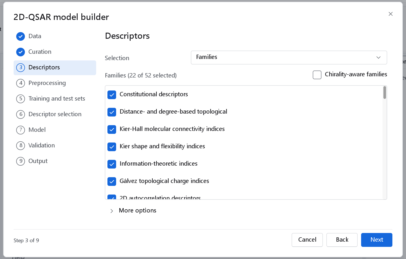
| Control | What it does |
|---|---|
| Selection | Families (the list), Named preset (the chirality-aware 2D and 3D presets), Identifiers (a list of descriptor names) or Everything (every registered descriptor). |
| Chirality-aware families | Adds or removes the seven chirality-aware 2D families. Not part of any recipe; tick it for a set that holds stereoisomers. |
| More options | Largest fragment only (off), Compute missing charges (on), Parallel (on). |
More families are not automatically better. Every column a model sees is a chance to fit noise, and the fewer compounds you have the more this matters. Add 3D families only when the structures have meaningful 3D coordinates.
4. Preprocessing
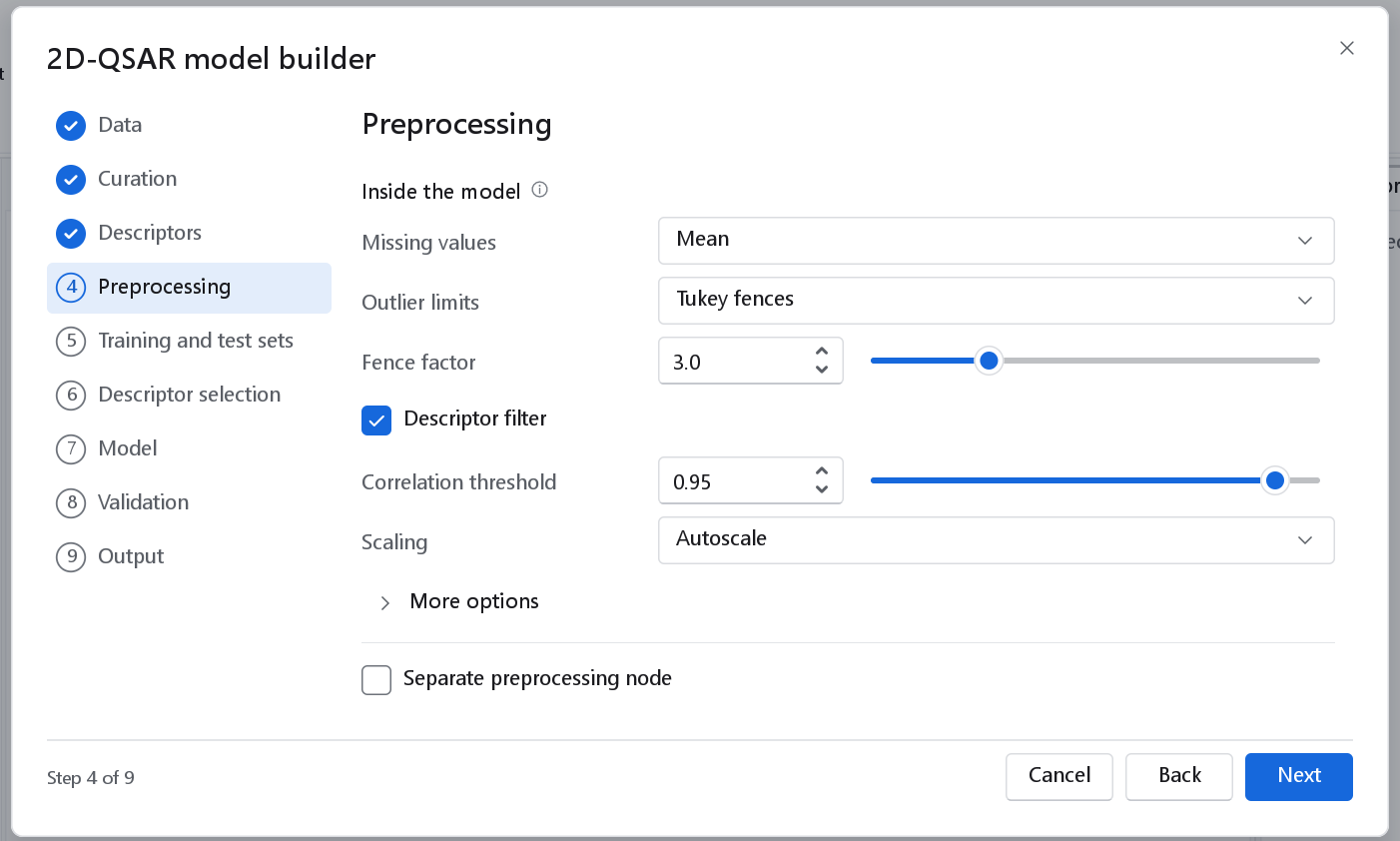
Missing values, outliers, redundant columns and scale are dealt with inside the model. These steps are fitted on the training compounds, fitted again inside every cross-validation fold and every Y-randomisation, and stored in the model bundle. Two things follow. The validation statistics include every fitted step, so no held-out compound influences any of them. And a saved model treats the descriptors of a new compound exactly as it treated its training set.
| Control | Choices | Recipe default and when to change it |
|---|---|---|
| Missing values | None, Mean, Median, k nearest neighbours | Mean. Median for skewed descriptors; with None a training node refuses a table with gaps. |
| Outlier limits | None, Tukey fences | Tukey fences for the linear recipes, none for forests. A value beyond Q1 - k IQR or Q3 + k IQR of the training compounds is set to the fence, so one extreme compound cannot dominate a linear model. Trees do not need it. |
| Fence factor | 0.5 to 10, shown with Tukey fences | 3.0. Smaller values clip more. |
| Descriptor filter | check box | On for the linear recipes. Drops constant descriptors and, of two descriptors correlated above the threshold, the one less correlated with the response. |
| Correlation threshold | 0.5 to 1, shown with the filter | 0.95. Lower it (0.9) for an MLR model, where collinear descriptors make the coefficients unstable. |
| Scaling | None, Mean-centre, Autoscale, Range [0, 1], Range [-1, 1], Pareto | Autoscale for PLS, so that every descriptor has the same weight; none for forests and for an MLR equation that should stay in descriptor units. |
Separate preprocessing node, off by default, adds a Preprocess descriptors node between the split and the model, fitted on the training rows. It imputes and filters columns but never scales, because values scaled outside the model would not be part of the saved bundle. The automatic model search is the one case that needs it, since its search has no imputation of its own, so the box is ticked and locked there.
5. Training and test sets
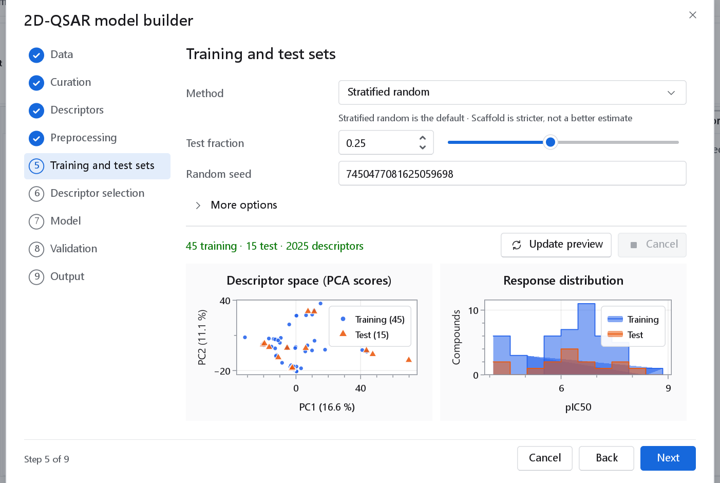
External validation needs compounds the model never saw. The split is a node of the workflow and is reproduced exactly whenever the workflow runs with the same seed.
| Method | How the test set is chosen | When to use it |
|---|---|---|
| Random | A seeded random draw of the test fraction. | Large sets with an even spread of activity. |
| Stratified random (the default) | The compounds are sorted into bins of equal frequency by activity (5 strata by default; by class for a classifier) and the test fraction is drawn from every bin. | The method the split node, the wizard and the recipes start from: test and training sets cover the same activity range, which the external criteria assume. |
| Kennard-Stone | A max-min distance design: the training set is picked to cover the descriptor space, and the remaining compounds form the test set. | Small sets where every region of chemical space must be in the training set. The test set is then easy, which flatters the external statistics. |
| DUPLEX | Snees alternating max-min design: training and test sets both span the descriptor space. | Like Kennard-Stone, with a more representative test set. |
| Sphere exclusion | Diversity sampling after Golbraikh and co-workers: a selected compound joins the training set and the compounds inside its sphere of radius R = c (V/N)1/K are shared between test and training up to the test fraction, with c the Dissimilarity (0.5). | Diverse libraries; c controls how close test compounds lie to training compounds. |
| Activity-sorted | The compounds are sorted by activity and every k-th compound (4 by default) is a test compound. | Small congeneric series; reproducible without a seed. |
| Cluster-based | The compounds are grouped into k-means++ clusters (5 by default) and every cluster contributes to the test set in proportion to its size. | Sets made of distinct chemical series. |
| Scaffold | The Bemis-Murcko scaffold of every compound is computed and each scaffold goes whole to the training set or to the test set, so no scaffold of the test set occurs in the training set. Largest first lets the common scaffolds train and tests on the rare ones; Balanced random draws the test scaffolds with the seed. Generic scaffolds groups frameworks that differ only in atom types or bond orders. | When a journal or a reviewer asks for a scaffold-disjoint test set, and as a stricter test of a model meant for a new chemical series. It does not give a more honest internal estimate than stratified random: on 45 independent data sets its estimate was the closer of the two to the external result on 21 of them, which is 47 % and no better than chance. On a congeneric series the option means little, since a scaffold test set could not be formed at all on 22 of 73 data sets, every one of them congeneric. |
| From a property | A column of the file names the set of every compound. | A published split, or the Training and Test marks set in the spreadsheet. |
| No test set | Every compound trains the model. | Only when the model will be validated on a separate external file; the external criteria are then not available. |
| Control | Default and when to change it |
|---|---|
| Method | Stratified random in every recipe. |
| Test fraction | 0.25, from 0.05 to 0.5. A quarter is the usual compromise; below about 40 compounds a test set of 10 or fewer gives noisy statistics, and cross-validation carries more of the weight. |
| Every k-th compound | Activity-sorted only: 4, from 2 to 10. |
| Clusters | Cluster-based only: 5, from 2 to 20. |
| Random seed | One seed for the split. Change it to check how much the statistics depend on the particular split; keep it to reproduce a result. |
| More options | Distance for the distance-based designs (Euclidean on autoscaled descriptors by default, or range-scaled, raw or Mahalanobis), Strata (5), Dissimilarity (0.5) and Limit outliers for distances (off). |
The preview computes the descriptors once and shows the split as it will be made: the PCA scores of the descriptor space (Jolliffe, Principal Component Analysis, 2nd ed., 2002) and the activity distribution of both sets. It warns about test compounds outside the training activity range, which the external criteria punish. Cancel stops a preview that takes too long. The number of training compounds it counts also sizes the recipe: below 40 the validation switches to leave-one-out.
How precisely a test statistic can be read
A test set of a 50-compound series holds about a dozen compounds, and an R2 or an RMSE measured on a dozen compounds cannot be located to better than tens of per cent. Measured on 50 independent series, the test estimate of the default recipe is unbiased in direction (median gap +0.029 against the result on compounds held back from the whole study) but its median absolute gap is 0.290, about 30 % of the value (see What has been validated).
A split the data already carry
The method From a property takes the two sets from a column of the file instead of making them: a published split, or the Training and Test marks you set in the spreadsheet. An edited dataset is handed to the wizard with its marks in the column set. Nothing is random here, so the page shows no test fraction and no seed.
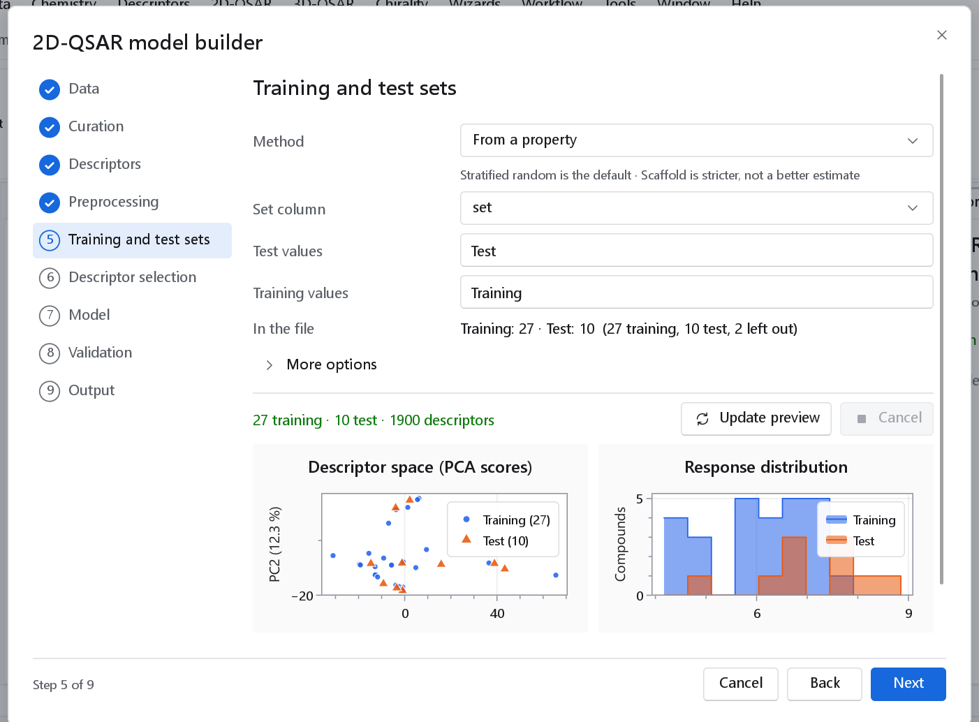
set. In the file counts the values the column holds and the result: 27 training, 10 test and 2 compounds left out because their value is in neither list.| Control | Meaning |
|---|---|
| Set column | The column that names the set of each compound. |
| Test values | The values that mean test set, separated by commas and compared without regard to case. |
| Training values | The values that mean training set. Empty: every compound that is not a test compound trains. With a list, a compound with another value is left out of the model. |
| In the file | The values found with their counts, and how many compounds fall into each set. |
6. Descriptor selection
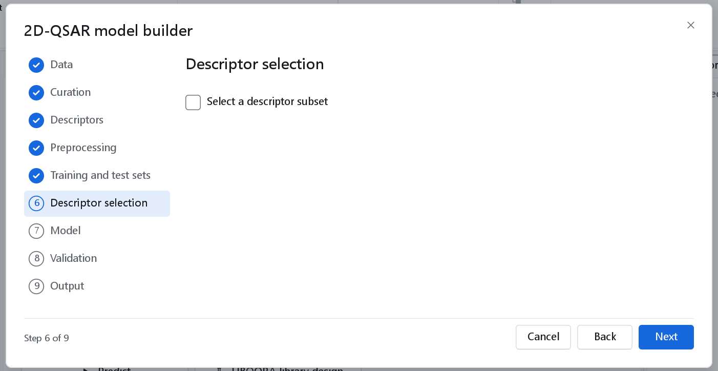
Off by default: PLS and the forests handle many descriptors, and the descriptor filter removes the redundant ones. Switched on with Select a descriptor subset, the selection becomes part of the model: the search runs on the training compounds and again inside every cross-validation fold and every Y-randomisation, so the reported statistics include the selection. A selection made once on all training compounds before cross-validation would make Q2 too optimistic; the wizard does not offer that route.
| Control | Choices and default |
|---|---|
| Method | Genetic algorithm (MLR), Genetic algorithm (PLS), Forward stepwise, Floating forward, Mutual information. The genetic algorithms are scored by the leave-one-out Q2 of the model they wrap. |
| Maximum descriptors | One descriptor per five training compounds, six at most, the usual upper limit for an MLR equation (Topliss and Costello, J. Med. Chem. 15:1066, 1972). |
| GA generations, GA population | 40 and 30, for the genetic methods. More options: GA runs (1). |
7. Model
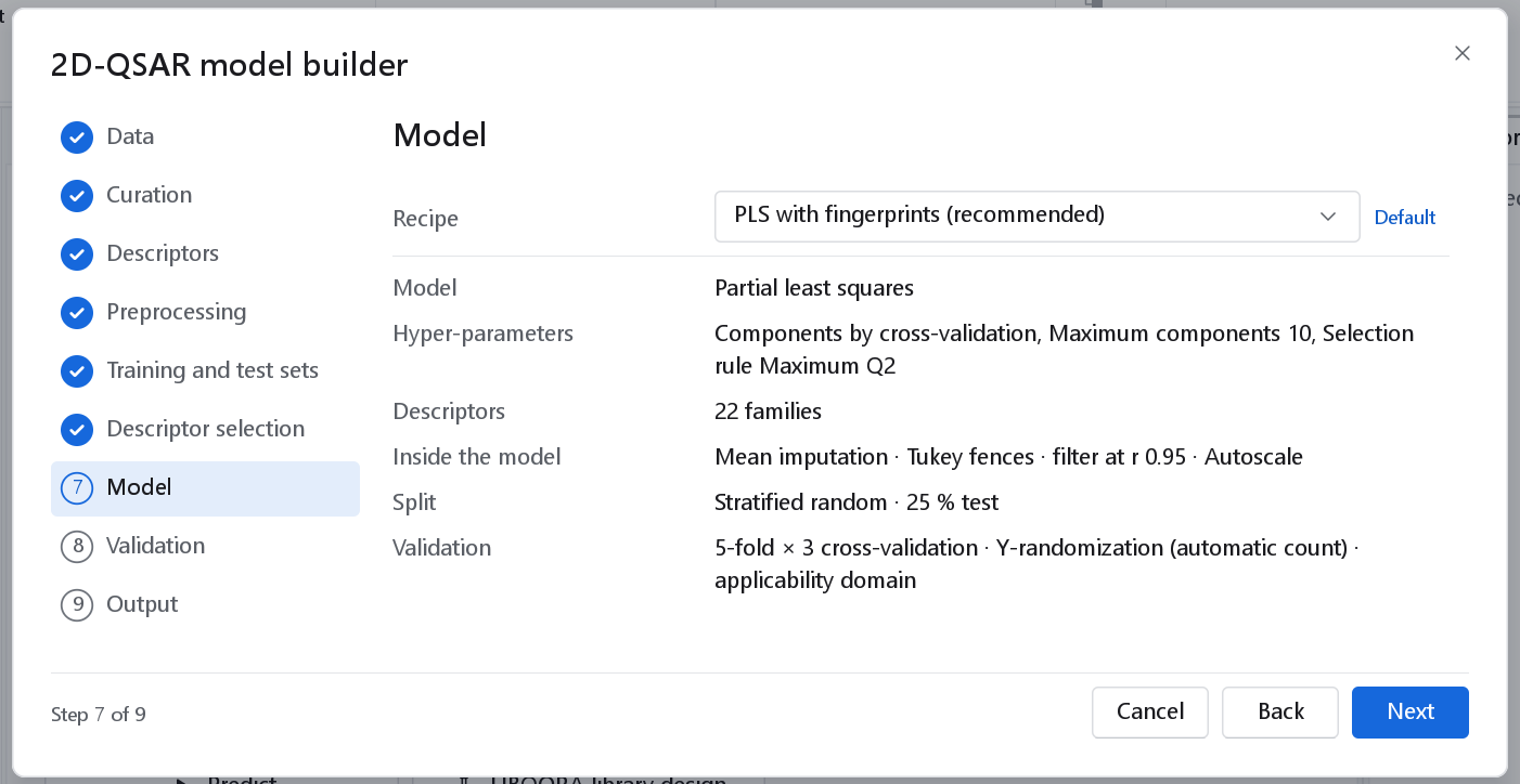
The first control of the page is the Recipe. A recipe is a complete choice of descriptors, preprocessing inside the model, model and hyper-parameters, split and validation protocol; the shipped workflow templates are built from the same recipes, so a wizard result and a template result are the same analysis. The page shows the recipe in effect and what it builds. It is tagged Default until you choose one, and Modified once a setting on any page differs from the recipe; the tooltip of Modified lists what differs and Restore sets it back.
| Recipe | What it builds | When to use it |
|---|---|---|
| PLS with fingerprints (recommended) | PLS on the 19 classical families and the three fingerprints, components chosen by cross-validation (Maximum Q2, at most 10), mean imputation, Tukey fences, filter at r 0.95, autoscaling. Domain by leverage in the latent space or fingerprint Tanimoto distance. | The default for regression. It was the most accurate recipe in the comparison of the recipes. |
| PLS on classical descriptors | The same PLS on the 19 classical families alone (904 columns). Domain by leverage or kNN distance over the model columns. | When every descriptor of the model must be individually interpretable, and for small sets, where a 3 976-column table invites overfitting. On the shipped acetylcholinesterase template it ran in about 1 s against about 15 s for the default. |
| Random forest with fingerprints | A forest of 500 trees on the 22 families, mean imputation, no limits, filter or scaling. Domain by fingerprint Tanimoto distance. | A non-linear alternative when PLS leaves structure in the residuals. |
| Interpretable (MLR equation) | A genetic algorithm picks a handful of classical descriptors (one per five training compounds, at most six) for an MLR equation in descriptor units, inside the model. Domain by leverage, kNN distance, descriptor range and PCA box. | Small congeneric series that need an explicit equation. Clearly less accurate than PLS. |
| Automatic model search | A search over model families and descriptor subsets (regression only). See Comparing models. | When no model family is preferred. |
| Custom | Your own list of models, starting from the values of the recipe that was in effect. | Several models side by side, or hyper-parameters of your own. |
Evidence for the default. The recipes were compared on twelve data sets (the shipped acetylcholinesterase, ESOL, FreeSolv and hERG sets and eight sets of Sutherland and co-workers): PLS with fingerprints had a mean Q2 of 0.608 against 0.554 for PLS on classical descriptors. On the shipped acetylcholinesterase template (322 training and 107 test compounds, three repeats of 5-fold cross-validation) it gives Q2 0.5565 and Q2F1 0.5019 against 0.4214 and 0.3874, and still fails 12 of the 19 acceptance criteria on that set. These sets were the ones the recipes were chosen on, so the figures show what the recipe reports, not an independent confirmation; see Accuracy and validation.
Custom: choosing models and hyper-parameters
Custom unlocks the list Models (N selected). Tick one or more models: each becomes its own pair of training and validation nodes on the same descriptors and the same split, and gets its own dashboard. The first model is the primary one, marked (primary): it feeds the report and the dashboard that is in front; Make primary changes it. The Parameters panel has one section per model with number fields and sliders over the offered range, check boxes and drop-downs. Less common parameters are under Advanced (n), and Reset to defaults removes every change. The defaults below are those of the model; a recipe may set others (the default recipe sets PLS to at most 10 components chosen by Maximum Q2).
| Model | Main hyper-parameters (default) | Notes |
|---|---|---|
| Partial least squares | Components (0 = choose by cross-validation), Maximum components (15), Selection rule (Wold R criterion; Maximum Q2; Q2 increment), Cross-validate (on), CV groups (7; 0 = leave-one-out), X scaling (Autoscale). Advanced: algorithm NIPALS or SIMPLS, Wold R threshold 0.95, Q2 increment limit 0.0975, Y scaling, random CV groups, tolerance. | The internal cross-validation only chooses the number of components; the validation page does the validation. |
| Multiple linear regression | Intercept (on), Confidence level (0.95). | Needs few, non-collinear descriptors: use it with descriptor selection. |
| Stepwise MLR | Direction (Both), Criterion (Partial F; p-value, AIC, BIC), F to enter (4.0), F to remove (3.9), p to enter (0.05), p to remove (0.10), Maximum descriptors (0 = automatic). | |
| Ridge regression | Automatic penalty (on, by generalised cross-validation), Penalty (1.0), Standardise (on). | Keeps every descriptor and shrinks the coefficients. |
| Elastic net / LASSO | L1 fraction (1.0 = LASSO), Cross-validate penalty (on), CV folds (10), Penalty rule (Minimum CV error; One standard error), Standardise (on). | Sets most coefficients to zero: a sparse linear model. |
| Principal component regression | As PLS without the algorithm choice. | |
| Random forest | Trees (500), Features per split (Automatic: p/3 for regression), Maximum depth (0 = unlimited), Minimum split size (2), Minimum leaf size (5), Bootstrap (on), Sample fraction (1.0), Out-of-bag estimate (on), Permutation importance (off). | Robust default for non-linear relationships. |
| Extra trees | As the random forest, with random thresholds, no bootstrap, minimum split size 5 and minimum leaf size 1. | |
| Gradient boosting | Loss (Squared error; Absolute error, Huber), Boosting rounds (500), Learning rate (0.05), Tree depth (3), Row subsample (0.8), Minimum leaf size (5), Early-stopping patience (20). | Often the most accurate tree model; tune the learning rate and the rounds together. |
| Support vector regression | Kernel (Gaussian (RBF); Linear, Polynomial, Sigmoid, Tanimoto), C (1.0), Gamma (0 = 1/p), Formulation (Epsilon-SVR; Nu-SVR), Epsilon (0.1), X scaling (Autoscale). | The Tanimoto kernel suits fingerprint columns. |
| k nearest neighbours | Neighbours (5), Automatic k (off, up to 15), Distance (Euclidean; Manhattan, Chebyshev, Cosine, Tanimoto), Weighting (Uniform; Inverse distance), X scaling (Autoscale). | A local model; useful as a baseline. |
| Gaussian process | Kernel (Gaussian (RBF); Matern 3/2, Matern 5/2), Optimise kernel (on), One length scale per descriptor (off), Length scale (1.0), Noise variance (0.1), Restarts (3). | Gives a standard error with every prediction. Slow above a few thousand compounds. |
| Neural network | Hidden layer 1 (64), Hidden layers 2 and 3 (0 = none), Activation (ReLU), Learning rate (0.001), Maximum epochs (500), Batch size (32), L2 penalty (0.0001), Dropout (0), Early stopping (on). | Needs many compounds. |
| Regression tree | Maximum depth (0), Minimum split size (2), Minimum leaf size (1), Pruning (None; Fixed alpha, CV minimum, CV one standard error). | One readable tree; rarely the most accurate model. |
Automatic model search
With the recipe Automatic model search the page shows the search instead of one model: Training/test splits (3), Tuning iterations (8 in the wizard), Consensus members (3), and under Search options the test fraction of each internal split (0.25), Stratified splits (on), Stop dominated candidates (on), Time budget (s) (0, no limit) and Fit on test rows too (off). The Descriptor selection page and the in-model preprocessing are skipped, the separate preprocessing node is switched on, and the outer test set is 0.2 of the compounds. What the search does, and why the test set never takes part in it, is explained in Comparing models.
8. Validation
| Option | What it does | Default and when to change it |
|---|---|---|
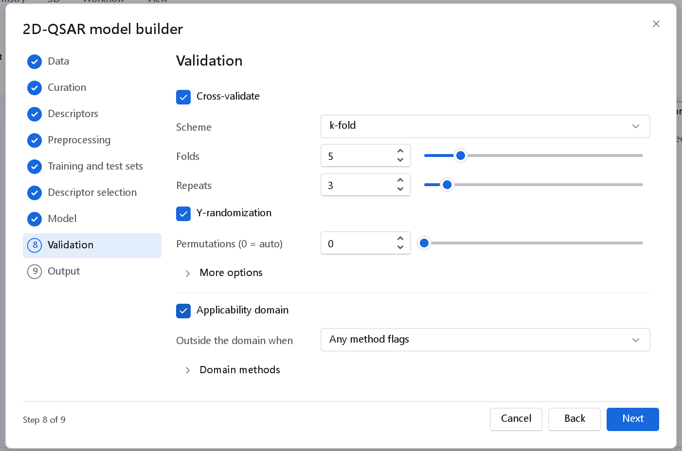
| Cross-validate | Estimates how the model predicts compounds it was not fitted on, from the training set alone. | On. |
| Scheme | Leave-one-out, k-fold, Leave-many-out, Bootstrap. | k-fold; leave-one-out below 40 training compounds, where folds of fewer than eight compounds give unstable statistics. Leave-one-out is optimistic for large sets. |
| Folds | k-fold only. | 5. |
| Repeats | Independent repetitions with new random folds; the statistics are computed from the held-out predictions averaged over the repetitions. | 3 (1 with leave-one-out). More repeats make Q2 less dependent on the fold assignment. |
| Y-randomization | The model is refitted on scrambled responses. A model whose scrambled twins score almost as well is fitting noise. | On. |
| Permutations (0 = auto) | 0 lets the validation choose: 50 when a permutation costs one fit, 20 when every permutation is cross-validated (the flexible learners). A number from 5 upwards is used as it is. | 0. |
| More options | Cross-validate each permutation (off): also gives the Q2 distribution of the permuted models for the linear models. It is always done for the flexible learners. | Off; costly. |
| Applicability domain | Fits the domain on the training compounds and stores it with the model. | On. |
| Outside the domain when | How the verdicts of the methods are combined: Any method flags, Most methods flag, All methods flag, A set number of methods flag, or one method alone (Leverage only, kNN distance only, Descriptor range box only, PCA bounding box only, DModX and Hotelling T2 only). | Any method flags: the strictest rule, which keeps a compound inside only when no method objects. |
| Domain methods | Node default | Meaning |
|---|---|---|
| Leverage / Williams | on (off in the forest recipe) | Leverage in the regression space; outside above h* = factor (p + 1) / n. |
| Leverage factor | 3.0 | The factor of h*. |
| kNN distance | on | Mean distance to the nearest training compounds. |
| Neighbours | 5 | |
| kNN distance measured on | Model columns | Model columns, Classical descriptors only, Fingerprint Tanimoto, or Classical descriptors or fingerprint Tanimoto. The fingerprint recipes use the Tanimoto distance: over a table of thousands of columns a Euclidean distance lets almost every foreign compound pass. |
| kNN distance threshold | Percentile of the training distances | Or Mean + Z standard deviations. |
| kNN percentile, kNN Z | 0.95, 0.5 | |
| PCA bounding box, Descriptor range box, DModX and Hotelling T2 | off | Switched on by the MLR recipe (the two boxes). |
| Significance level | 0.05 | For DModX and T2. |
| Methods needed to flag | 1 | For A set number of methods flag. |
With the fingerprint Tanimoto distance the domain of the default recipe kept 92.2 % of held-out test compounds inside and placed 99.4 % of compounds from unrelated data sets outside, over the benchmark data sets of the program's validation.
9. Output
| Option | Result | Default |
|---|---|---|
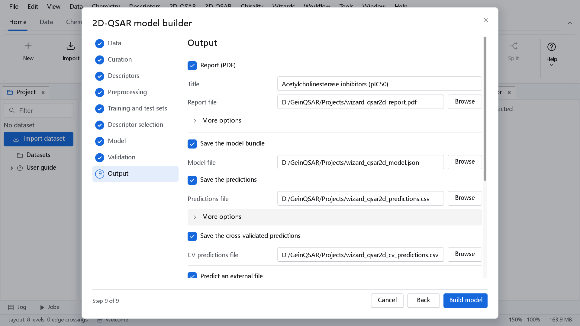
| Report (PDF), Title, Report file | The report following the OECD principles, with the metric table and the Y-randomisation runs. More options holds the rest of the report node, including its Word and Excel forms and the paper size. | On |
| Save the model bundle, Model file | The model with its descriptor names, the preprocessing fitted with it and its applicability domain, as a .json bundle. The prediction wizard applies it to new compounds. | Off. Tick it for any model you intend to use. |
| Save the predictions, Predictions file | Observed and predicted value, residual and domain verdict of every compound, as CSV. | Off |
| Save the cross-validated predictions, CV predictions file | The prediction of every training compound by a model fitted without it: the numbers Q2 is computed from. Shown with cross-validation on. | Off |
| Predict an external file | Applies the primary model to a second file of compounds that took no part in the modelling; every row is predicted and none is merged. A data page for that file and its predictions file appear below. | Off |
The workflow the wizard builds
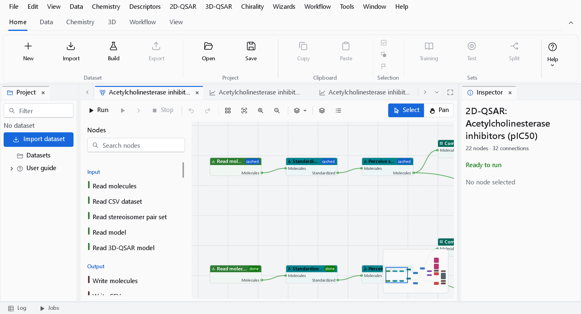
Build model writes the workflow, opens it on the canvas and runs it. Each page of the wizard became one or more nodes, with every value you saw as a parameter. Select a node to read or change its parameters in the inspector, then Run again; see The workflow canvas.
The OECD principles
The validation follows the OECD principles for (Q)SAR models (OECD, Guidance Document on the Validation of (Quantitative) Structure-Activity Relationship Models, ENV/JM/MONO(2007)2). Each principle is settled on one of the pages:
| Principle | Where it is settled |
|---|---|
| 1. A defined endpoint | Data page: the activity column, its units and transform. The report has a free-text endpoint field. |
| 2. An unambiguous algorithm | The workflow itself: every node and parameter, the recipe, the seeds and the program version are recorded in the report and the provenance. |
| 3. A defined domain of applicability | Validation page: the applicability domain, fitted with the model and stored in the bundle. |
| 4. Measures of goodness of fit, robustness and predictivity | Validation page and the split: R2, cross-validated Q2, Y-randomisation and the external test set statistics. |
| 5. A mechanistic interpretation, if possible | The coefficients, VIP scores and equation on the Descriptors tab of the dashboard, and a free-text mechanism field in the report. |