Contour maps and atom cubes
How to read a KEFRA contour map and an atom-class cube map, how the contour levels are chosen, how to set up the view, and how the figures for a paper are made.
A 3D-QSAR model can be drawn in space around a ligand, showing where the model predicts that more bulk, more positive charge, a donor or a hydrophobic group would raise or lower the activity. That picture is the reason most people build a 3D model at all, and it is also the easiest part of a study to over-interpret. A KEFRA model is drawn as contour lobes, one pair per field; an atom-based model is drawn as the cubes of its lattice.
What is mapped
An atom-based cube model has one coefficient for every lattice cube and atom class. A KEFRA model has no lattice coefficients: its kernel model is projected back into space as an activity field for each property, sampled on a lattice drawn for the map alone. Both are read in the same way.
For the cubes the mapped quantity is StDev x Coeff, the usual 3D-QSAR map convention: the regression coefficient of a lattice point multiplied by the standard deviation of the field at that point over the training set. It is the change in predicted activity when the field at that point rises by one training standard deviation, so it is large only where the molecules of the series differ and the difference matters (Cramer, Patterson and Bunce 1988). A bare coefficient is misleading, because lattice points differ enormously in how much they vary across the series; a point inside every molecule can have a large coefficient and no influence on any prediction.
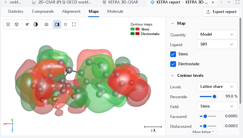
A map is read against a ligand. A green lobe next to a substituent says that a larger substituent in that direction is predicted to help; a yellow lobe says that the space is predicted to be full. The map describes the training series in the frame of its alignment: it says nothing about regions no training compound reaches, and a lobe where only one compound has an atom rests on that compound alone.
Colours
| Field | Favoured lobe | Disfavoured lobe |
|---|---|---|
| Steric | Green: more bulk raises the predicted activity. | Yellow: more bulk lowers it. |
| Electrostatic | Blue: more positive charge raises the predicted activity. | Red: more negative charge raises it. |
| Hydrophobic | Yellow: a hydrophobic group raises the predicted activity. | White: a hydrophobic group lowers it. |
| H-bond donor | Cyan: a donor raises the predicted activity. | Purple: a donor lowers it. |
| H-bond acceptor | Magenta: an acceptor raises the predicted activity. | Red: an acceptor lowers it. |
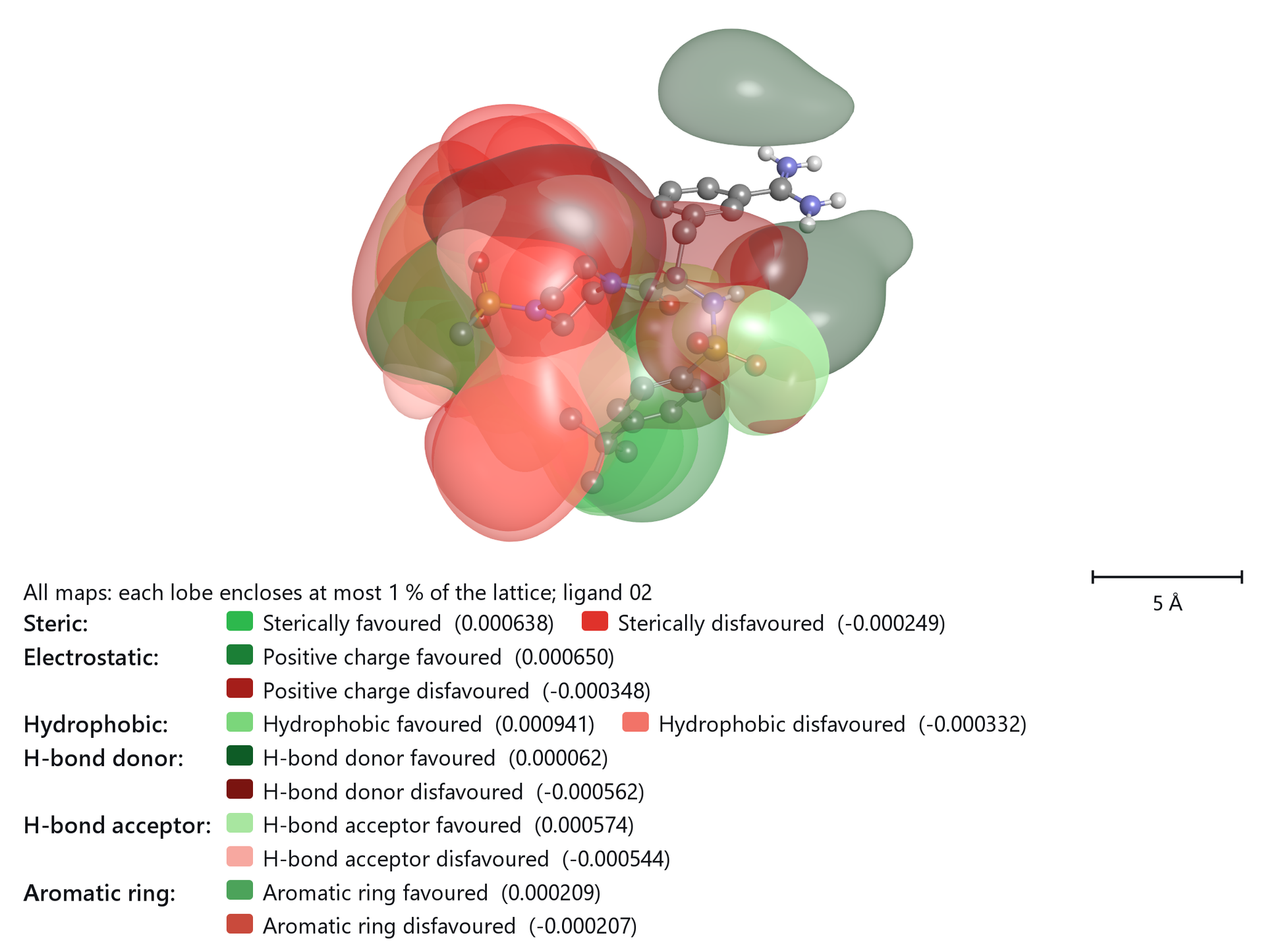
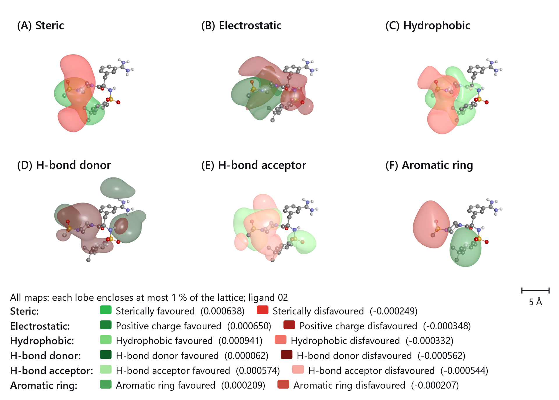
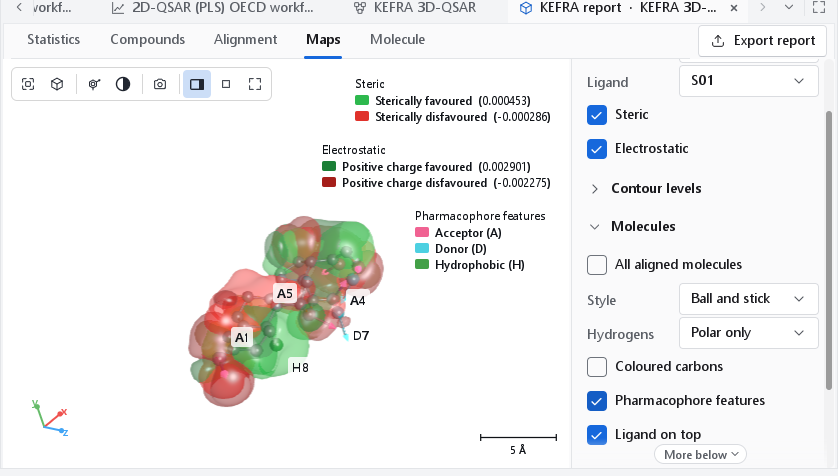
These are the colours of the Classic preset, the convention such maps are usually published in. It uses yellow and red twice (sterically disfavoured and hydrophobic favoured; negative charge favoured and acceptor disfavoured), which is harmless as long as every field has its own view. The Colours drop-down of the Appearance section offers three presets: Classic; Distinct, which gives every lobe of a view with several fields a colour of its own; and Activity (green / red), green where the property raises the predicted activity and red where it lowers it, every field in its own shade. Until you pick one, the program uses Activity. The legend always names the colours that are drawn and the iso-level of each lobe, so a reader never has to guess.
Contour levels
How the two levels of a field are chosen changes what a map shows more than anything else, so the definition is a control of its own (Levels in the Contour levels section) and is stated in the legend of every exported figure, for example "Steric (each lobe encloses at most 1 % of the lattice; ligand 02)". The report lists the definition and the two levels of every field.
| Definition | Meaning | When to use it |
|---|---|---|
| Lattice share | The default. Each lobe encloses the same small share of all lattice points: at the 99th percentile the top 1 % for the favoured lobe and the bottom 1 % for the disfavoured one. A lobe never encloses more than half of the points of its sign, so a field with few points of one sign still shows a lobe. Percentile runs from 90 to 99.9. | Almost always: it gives lobes of comparable size, about the volume of a substituent at 1 %, on every field. |
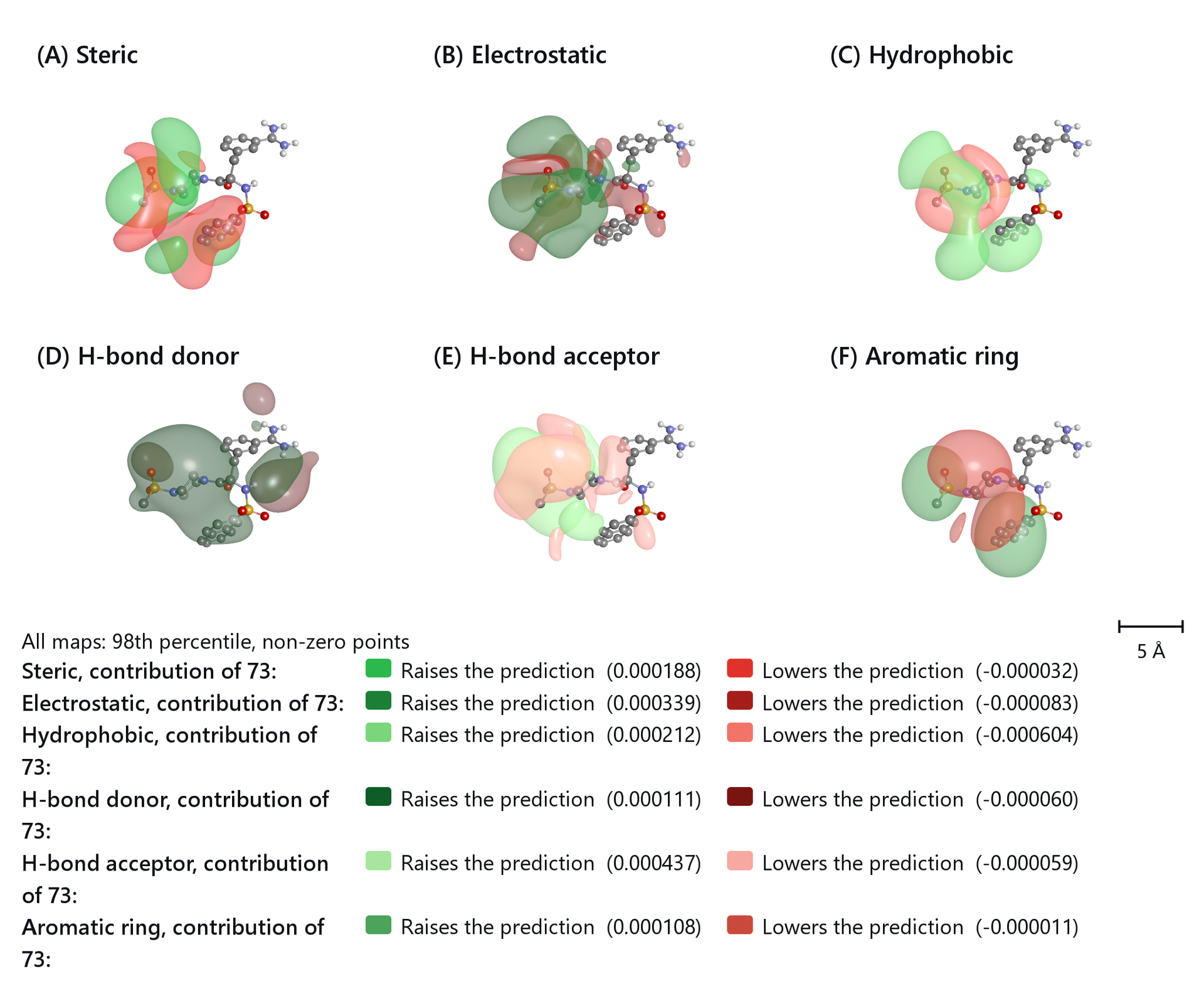
| Non-zero | The favoured level is the given percentile of the positive values, the disfavoured level the mirrored percentile of the negative values; only lattice points that carry a value count. Starts at the 70th percentile. | Contribution maps of one compound, where most points of one sign lie close to zero. |
| Classical | The 80th and 20th percentile of all lattice values, the usual 3D-QSAR definition. Starts at 80. | To compare with an older paper that used it. |
| By hand | The two levels are the values of the Favoured and Disfavoured sliders, in map units. Moving a slider selects this definition. | To show the same levels on two models. |
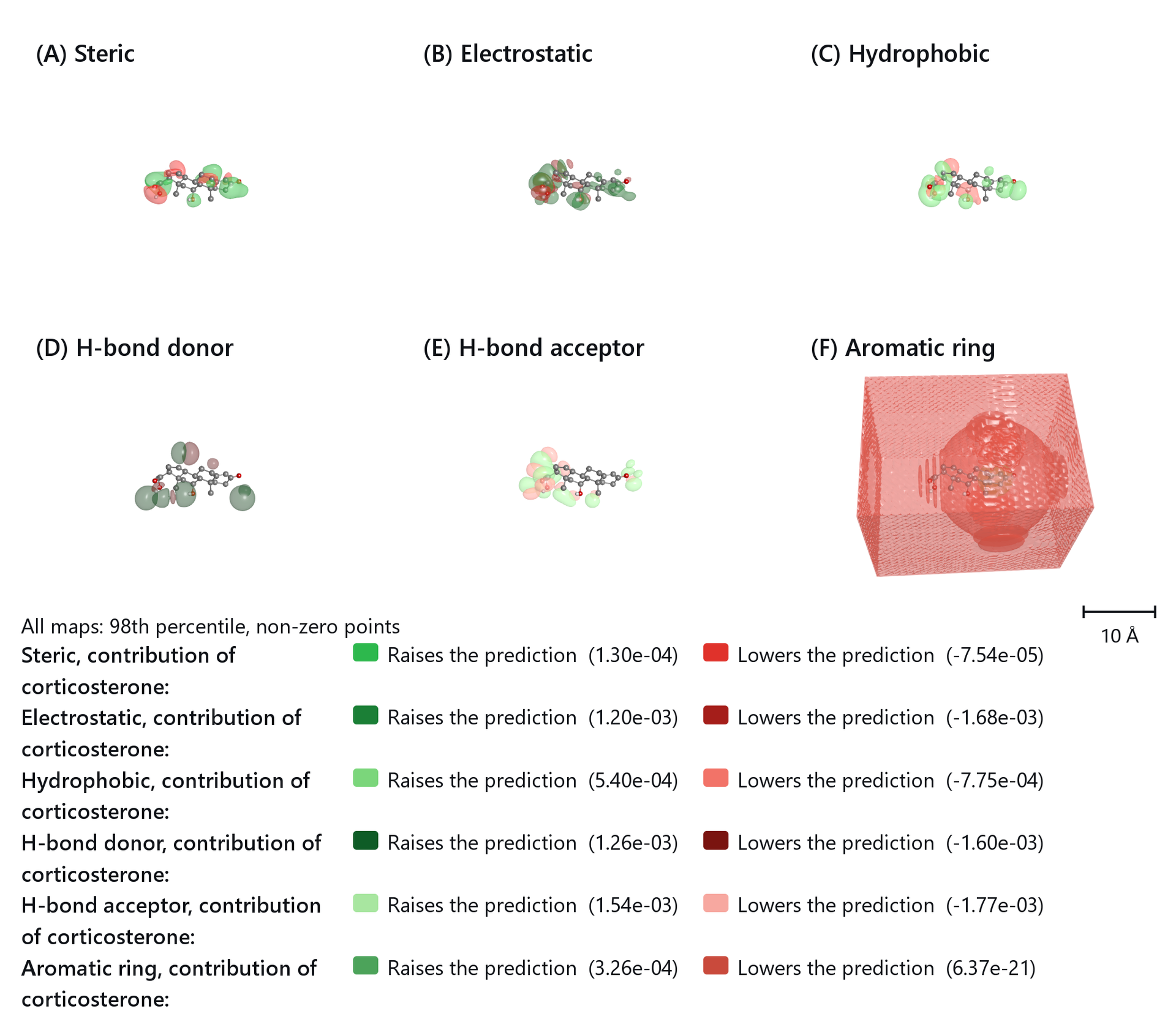
The default is a share of the lattice because maps differ in how much of the lattice they use. On a map that is non-zero at a few per cent of the lattice points the classical 80th and 20th percentile falls close to zero, and on a smooth map that is non-zero almost everywhere a percentile of the non-zero points encloses a third of the whole box; in both cases the lobes merge into a shell around the ligand. Field chooses which field's two levels the sliders show. When you describe a figure, quote the definition its legend gives.
The surfaces are not contoured directly on the lattice, which gives faceted shapes that depend on where the points fall. The lattice is refined with an interpolating cubic spline and the surfaces extracted by marching cubes with normals from the analytic gradient. For a Gaussian lobe sampled at 2 Å, the enclosed volume then deviates from the exact value by 0.1 %, against 21 % for direct contouring.
Contribution of one compound
With Quantity set to One compound and a compound chosen in Compound, the map shows where the compound's own field gains or loses predicted activity relative to the average training compound: (x - mean) x coefficient for the cubes, and for KEFRA the field of the compound minus the training mean, times the model. Summed over the map, the values give the prediction of the compound minus the mean training activity. The legend then reads Raises the prediction and Lowers the prediction. Because most points of one sign lie close to zero, these maps are best drawn with the Non-zero definition.
The steroid model
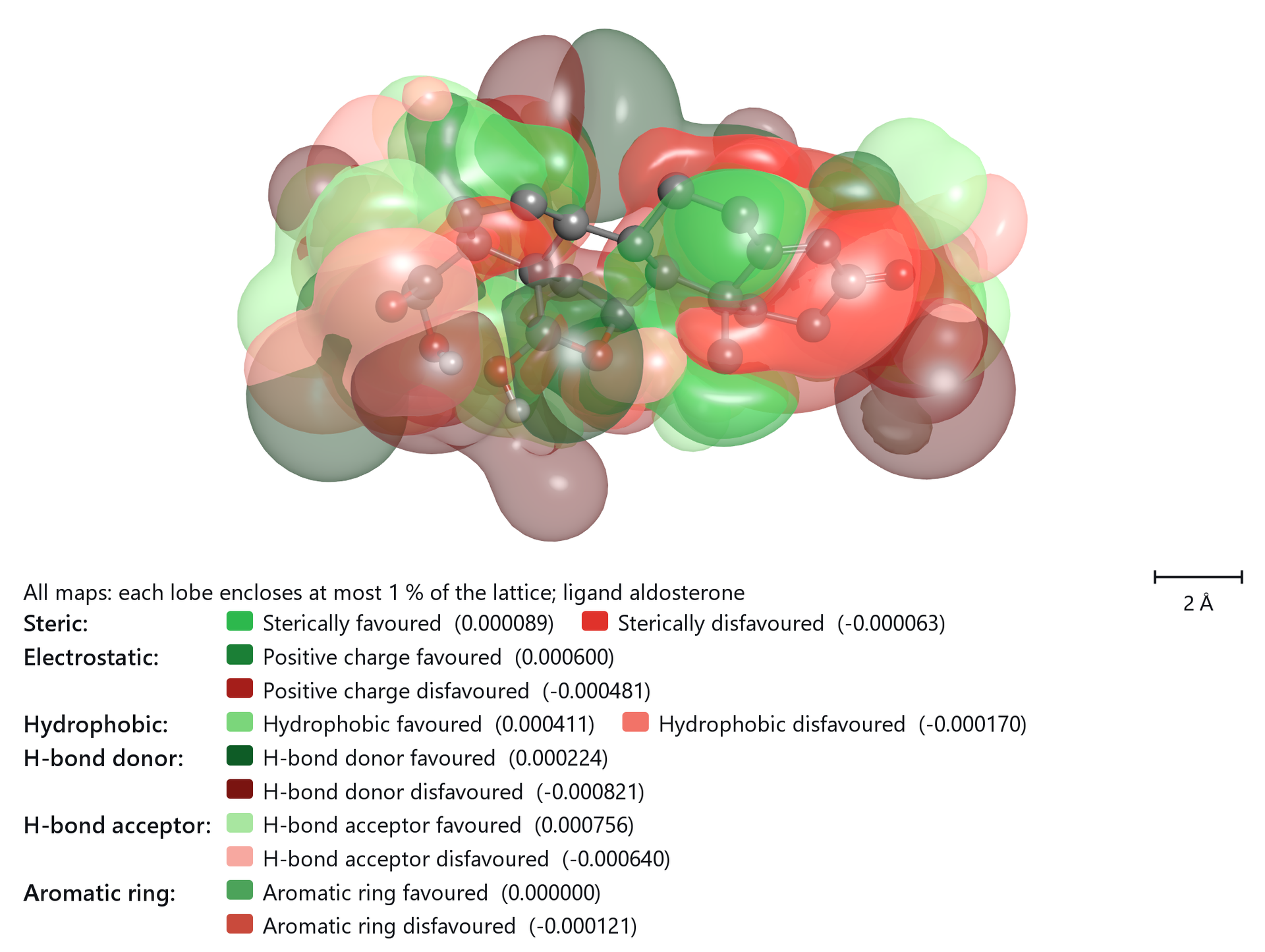
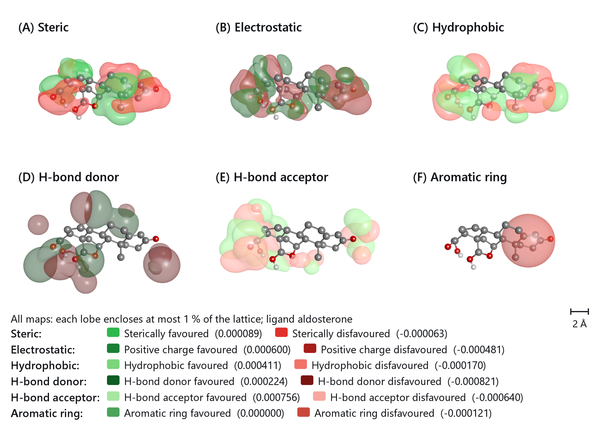
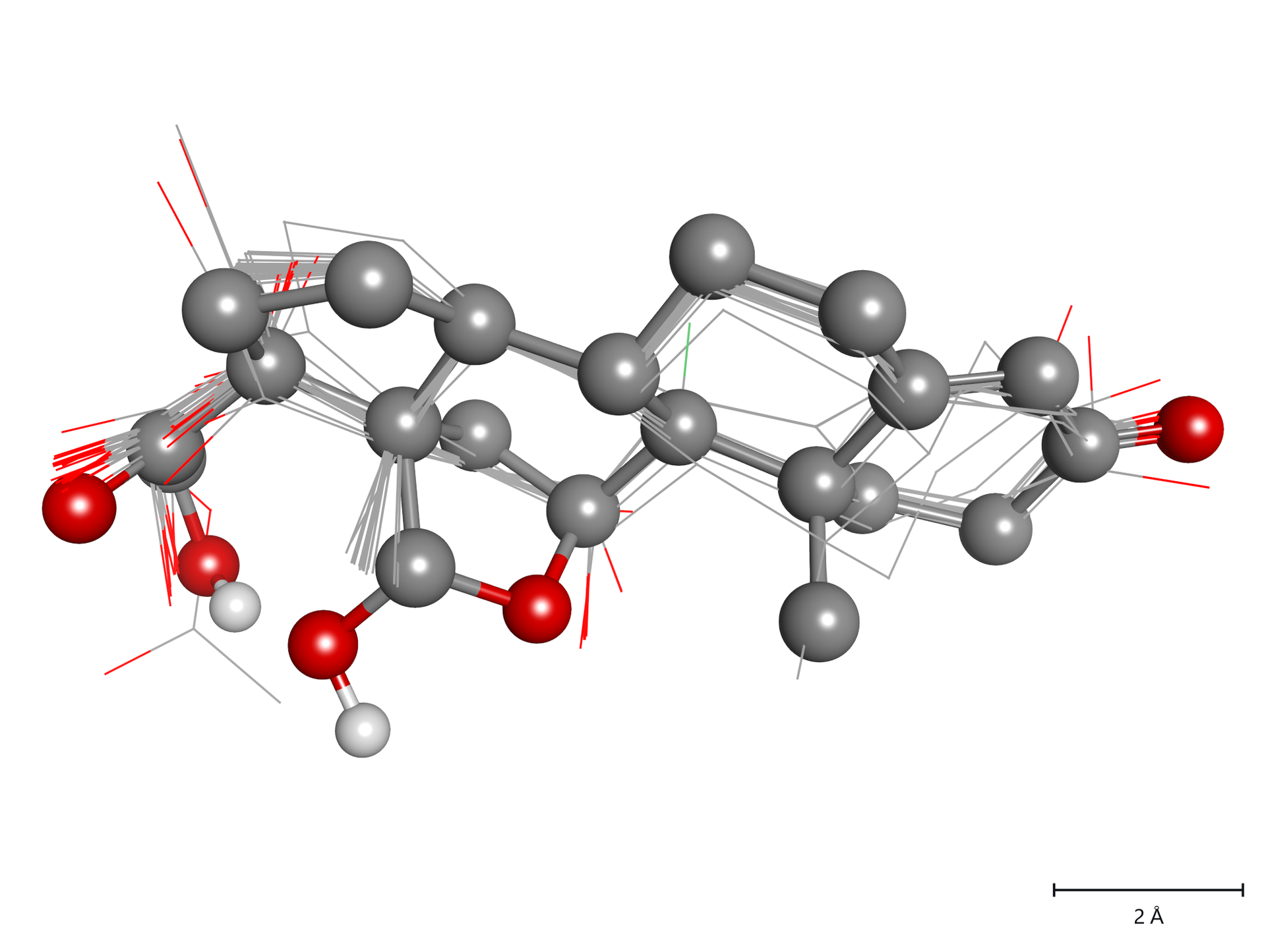
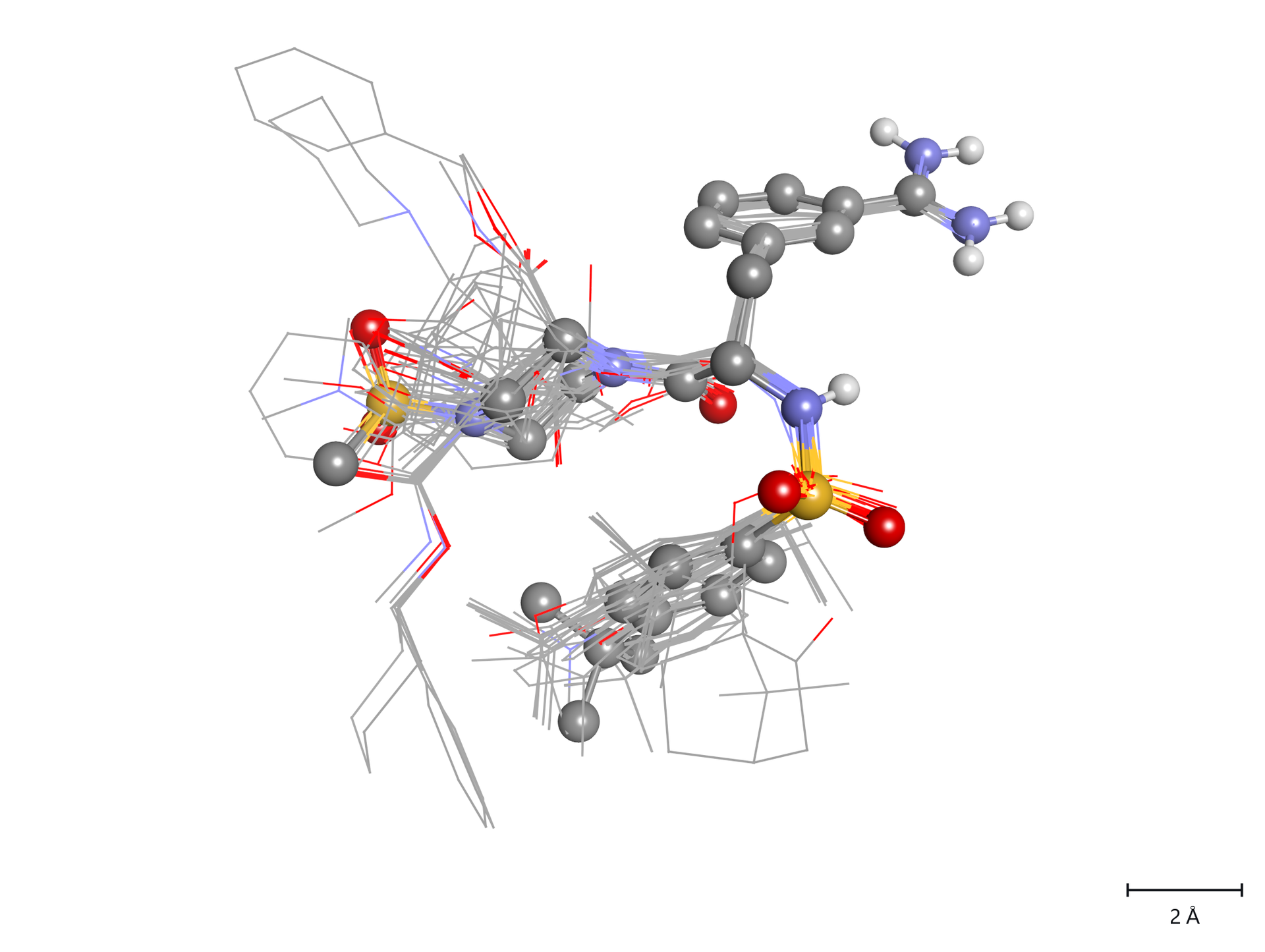
A figure of the alignment alone belongs next to every map in a paper: it shows where the series has atoms, and therefore where a lobe can mean something.
Atom-class cubes
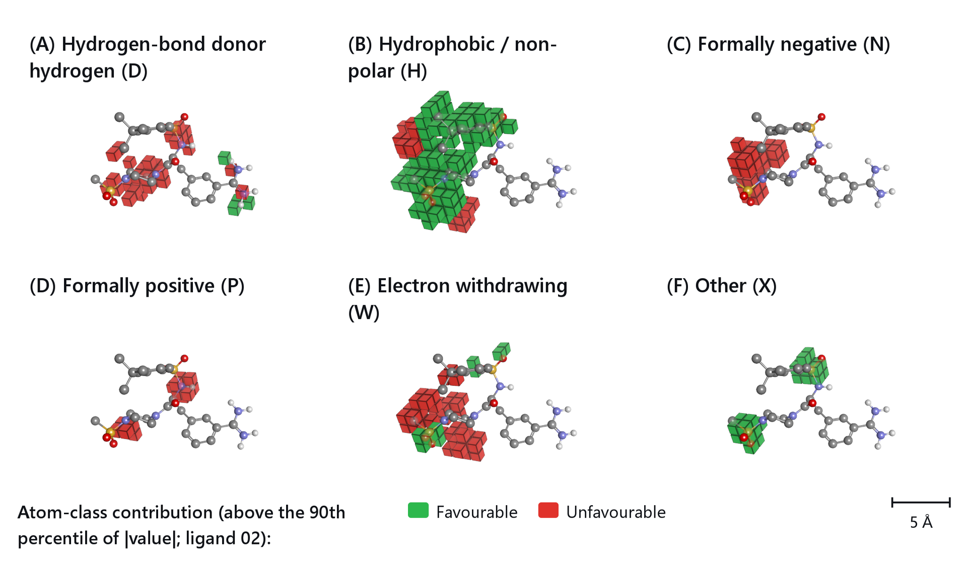
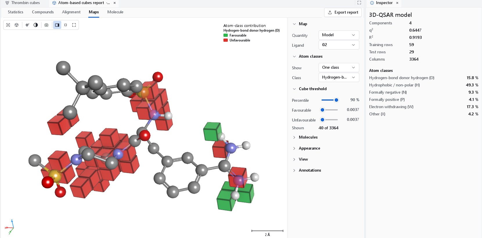
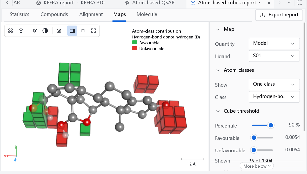
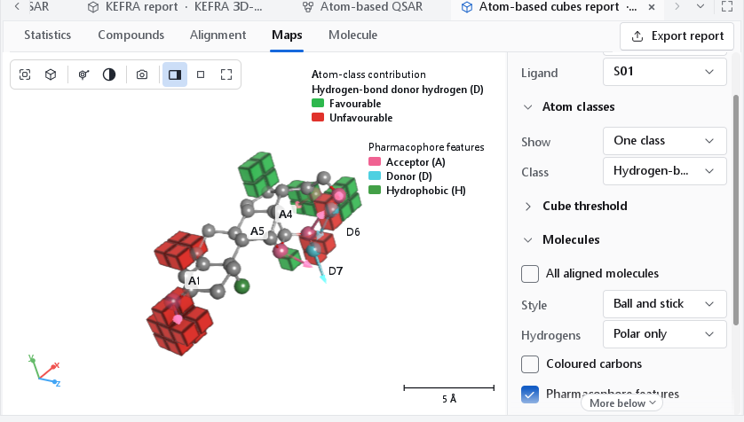
An atom-based model counts, for every cube of the lattice, the volume filled by the atoms of each of six classes. Its map draws the cubes themselves. Within a class, one colour marks cubes where an atom of that class raises the predicted activity (blue, Favourable) and the other where it lowers it (red, Unfavourable).
| Letter | Class | Atoms |
|---|---|---|
| D | Hydrogen-bond donor hydrogen | A hydrogen bonded to N, O, P or S. |
| H | Hydrophobic / non-polar | Carbon, hydrogen on carbon, halogen. |
| N | Negative ionic | A formally negative atom. |
| P | Positive ionic | A formally positive atom. |
| W | Electron withdrawing | Nitrogen or oxygen, which includes the acceptors. |
| X | Other | Everything else. |
The published class list overlaps (a carboxylate oxygen is both N and W), so each atom is assigned to one class by the priority N, P, D, W, H, X.
| Control | Default | Meaning |
|---|---|---|
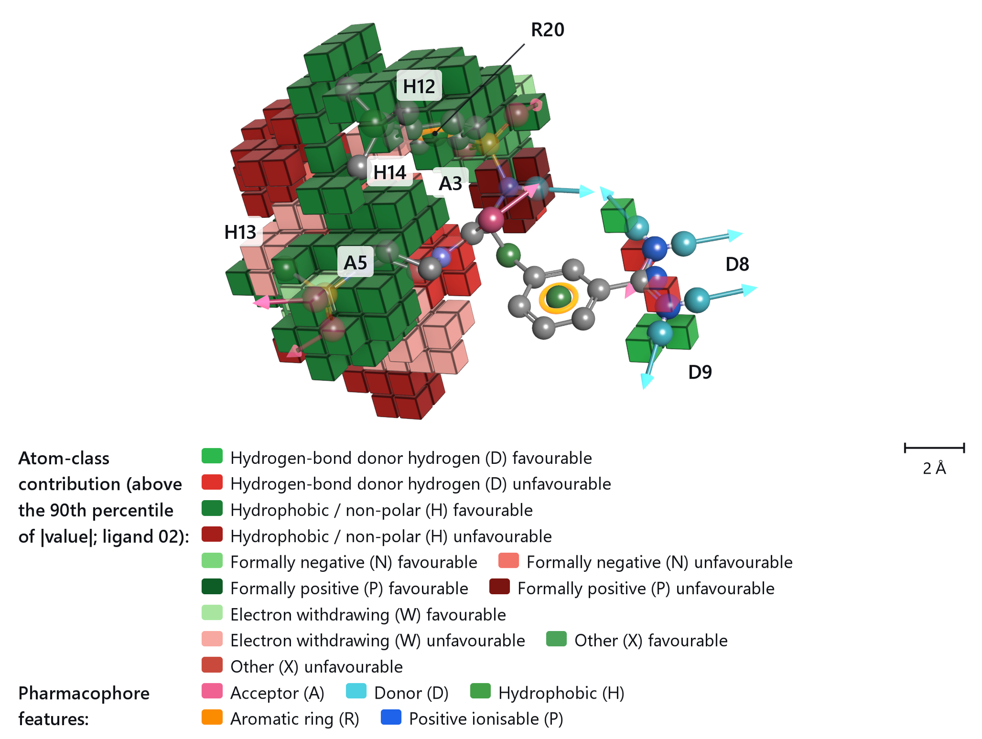
| Show | One class | One class: a single class in blue and red, the way atom-based maps are published, chosen in Class. All classes: every ticked class in its own colour pair. |
| Percentile | 90 % | Cubes below this percentile of |value| are hidden, so the default shows the strongest tenth of the model. An atom-based model has thousands of columns, and drawing more of them fills the view with a solid block. Moving it sets both thresholds. |
| Favourable, Unfavourable | The two thresholds separately: cubes at or above the first are drawn favourable, at or below minus the second unfavourable. | |
| Shown | The number of cubes drawn out of all cubes of the model. |
Cubes with the pharmacophore features of the ligand
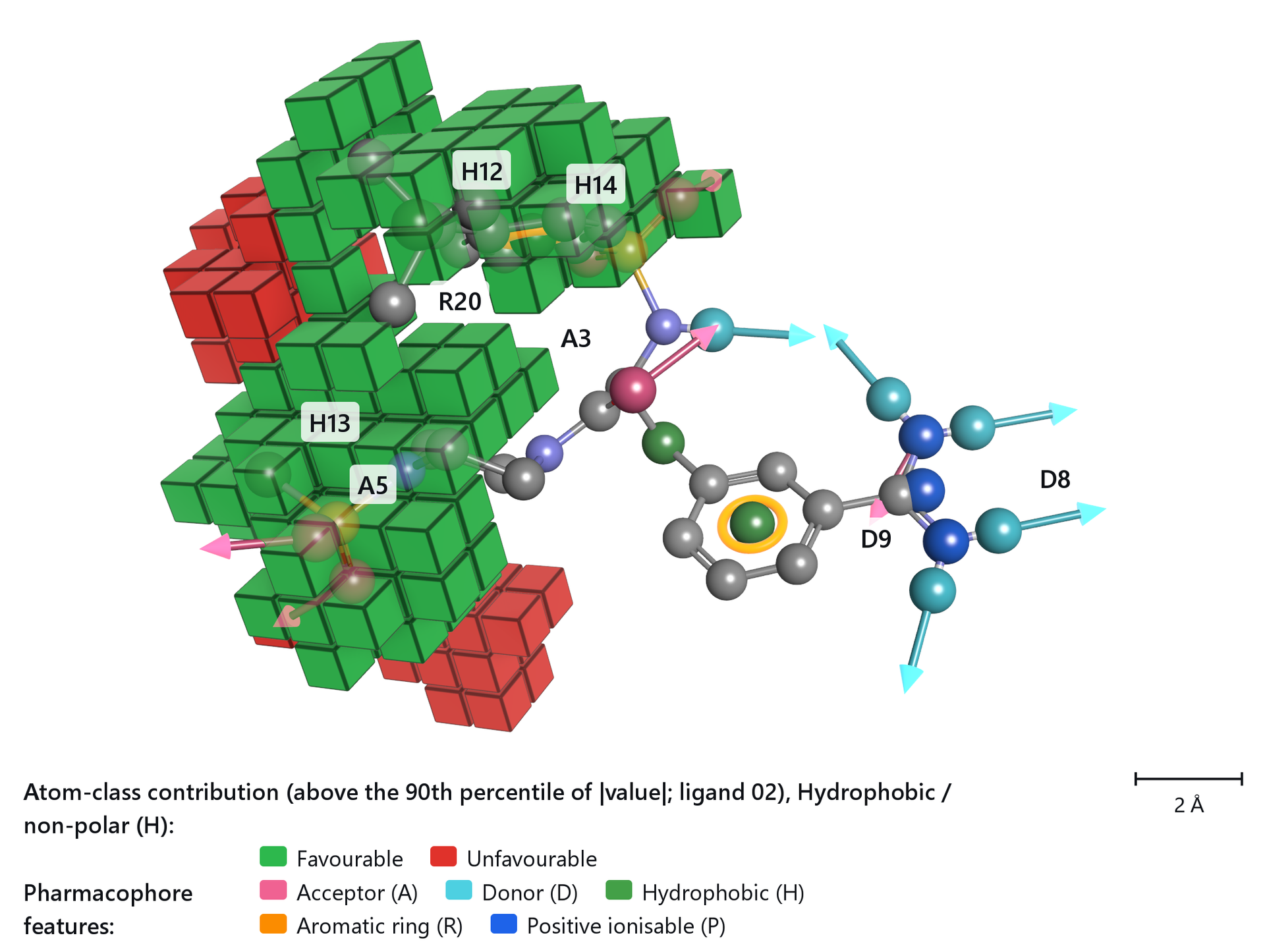
Pharmacophore features in the Molecules section perceives the acceptor, donor, hydrophobic, ionic and aromatic features of the ligand and draws them as glyphs over the map, so a cube or a lobe can be read against the feature that sits there. These are the features of that one ligand, not a pharmacophore hypothesis.
The display controls
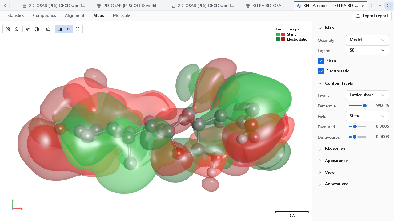
The Maps tab opens the way a map is usually published: smooth translucent lobes, the ligand as ball and stick with its polar hydrogens, the legend in the corner, no lattice box, and the camera on the best view of what is drawn, framed tightly. The panel beside the viewer has these sections.
| Section | Controls |
|---|---|
| Map | Quantity: Model or One compound. Compound: the compound of a contribution map. Ligand: the compound drawn inside the map, or None; it does not change the map. One box per field of a contour map. |
| Contour levels | Levels, Percentile, Field, Favoured, Disfavoured, as above. |
| Atom classes, Cube threshold | Cube maps only, as above. |
| Molecules | All aligned molecules: every aligned compound as thin lines. Style (default ball and stick) and Hydrogens (default polar only) of the ligand. Coloured carbons and Carbon colour: one colour for the carbons of the ligand instead of element grey. Pharmacophore features. Ligand on top (on): keeps the ligand readable through the map; on a dark background the map is thinned over the ligand, on a white or light background the ligand keeps its own colours and the part a lobe hides shows through. |
| Appearance | Contour maps: Colours (the presets above), Lobe values (off; see below), Style (Solid, Mesh, Dots), Opacity (0.78), Lattice box, and Own lobe colours with a Favoured and a Disfavoured colour for the field chosen under Contour levels. Cube maps: Opacity (1: solid), Fade distant cubes, Cube edges. |
| View, Annotations | As in every 3D view; see The 3D workspace. |
A control panel whose controls continue below its lower edge shows a More below sign until they have been scrolled into view, so a setting cannot be missed because the window is short.
How much each lobe is worth
A coloured lobe says where, not how much. Lobe values in the Appearance section labels every lobe with the contribution it makes to the predicted activity, compared with the average compound, and names the nearest atom and group of the ligand, and it lists the lobes in a table under the view with their map values. A label is plated green where the lobe raises the predicted activity and red where it lowers it, while the surfaces keep the colours of the field, so the direction and the field can be read at the same time.
The table holds the lobes that carry at least 1 % of the largest contribution, at most twenty of them, and the rest go to the Excel form of the report. That is what turns a map into a statement about a functional group: not that a region is favourable, but that this substituent in this position accounts for this much of the prediction.
Figures for a paper
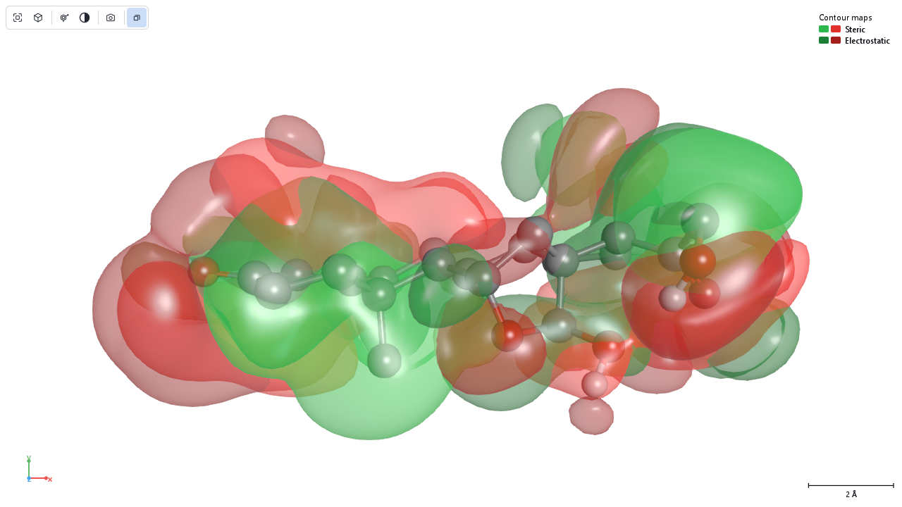
The camera button of the viewer toolbar opens the 3D figure dialog. The figure is rendered off screen at its own size and resolution, not copied from the screen, so it is sharp at any size, and the preview in the dialog is the same figure at a low resolution. The figures on this page were made that way, at 174 mm and 300 dpi. The choices that matter for a map:
- Layout Figure panels with One panel per Fields gives one panel per field of a contour map, each with a letter; Atom classes one panel per class of a cube map. The panels share one camera, so they can be compared region by region.
- Legend Automatic puts the legend below the scene when the figure is narrower than 120 mm or has several legends. The legend states the level definition and the ligand.
- Background White and Publication look give crisp outlines, contact shadows and print tone mapping.
- View state file also writes the camera and render settings of the figure, so the same figure can be made again after the model is rebuilt.
Every control of the dialog is described on Publication figures. A good caption names the model and its alignment, the ligand, the level definition and what the colours mean, which is everything the legend of the figure also carries.