The 3D-QSAR dashboard
What a 3D-QSAR run produced: the statistics and the chosen number of components, the per-compound predictions, the alignment the model rests on, the maps, and the contribution of each atom.
The dashboard opens when a 3D-QSAR workflow finishes, one per model: a run with KEFRA and the atom-based cubes opens two. It recomputes nothing. Every number is read from the output of the workflow, so the dashboard, the exported report and the files the workflow wrote always agree. The explanations are tooltips: rest the pointer on a card, a column heading or the help mark next to a section title.
| Tab | Shows |
|---|---|
| Statistics | The selected model as cards, the rule that chose the number of components, the statistics for every number of components, the model statistics, the field contributions, observed against predicted, and the Y-scrambling and bootstrap results when they were run. |
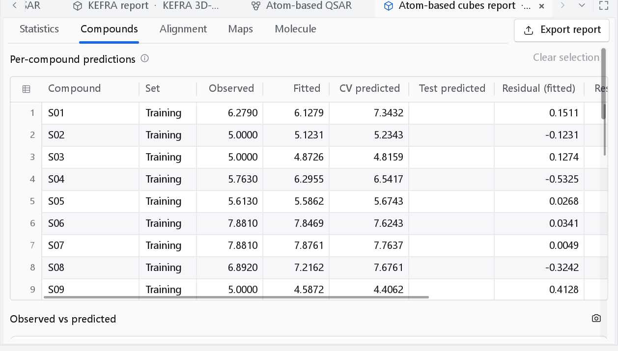
| Compounds | One row per compound with its set, observed and predicted values, and how far it reaches beyond the lattice. |
| Alignment | The alignment the model was built on, molecule by molecule. |
| Maps | The model as a 3D contour or cube map with a ligand inside it. |
| Molecule | One compound in 2D with its atoms coloured by their contribution to the prediction. |
Statistics
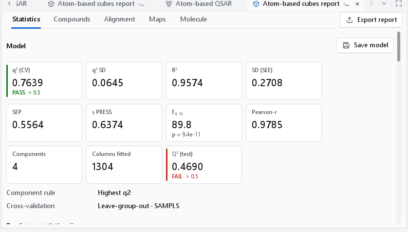
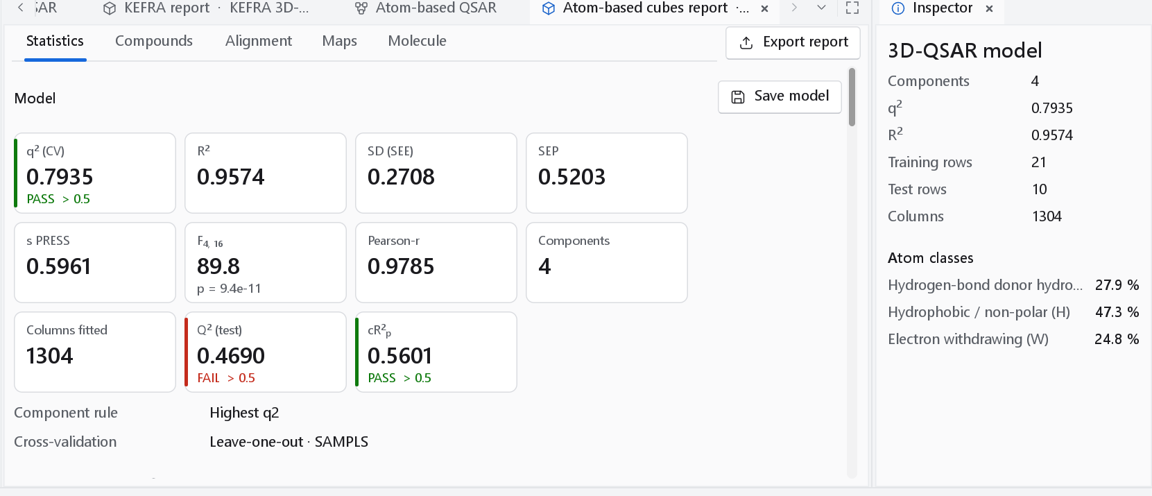
An atom-based cube model is a PLS model and has these cards:
| Card | Definition | Threshold |
|---|---|---|
| q2 (CV) | 1 - PRESS / SS from the cross-validation of the protocol (Cramer et al. 1988). | Above 0.5 |
| R2 | 1 - RSS / SS on the training set at the selected number of components. | |
| SD (SEE) | Standard error of estimate, sqrt(RSS / (n - A - 1)) for n compounds and A components. | |
| SEP | Standard error of prediction, sqrt(PRESS / n), from the cross-validation. | |
| s PRESS | sqrt(PRESS / (n - A - 1)), the cross-validated standard error the 3D-QSAR literature tabulates. | |
| q2 SD | Standard deviation of q2 over the repeats of a repeated cross-validation. Not shown for leave-one-out, which has none. | |
| F | Fisher F of the fit, (R2 / A) / ((1 - R2) / (n - A - 1)). | |
| Pearson-r | Correlation of observed and fitted activities. | |
| Components, Columns fitted | The number of PLS components and of lattice columns left after the filters. | |
| Q2 (test) | Q2F1 of the test set: 1 - PRESS(test) / SS of the test values about the training mean (Shi et al. 2001). | Above 0.5 |
| cR2p | R sqrt(R2 - mean R2 of the scrambled refits) (Mitra, Saha and Roy 2010). Shown when Y-scrambling was run. | Above 0.5 |
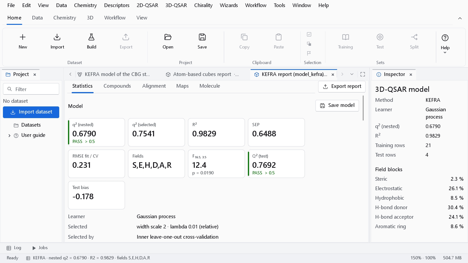
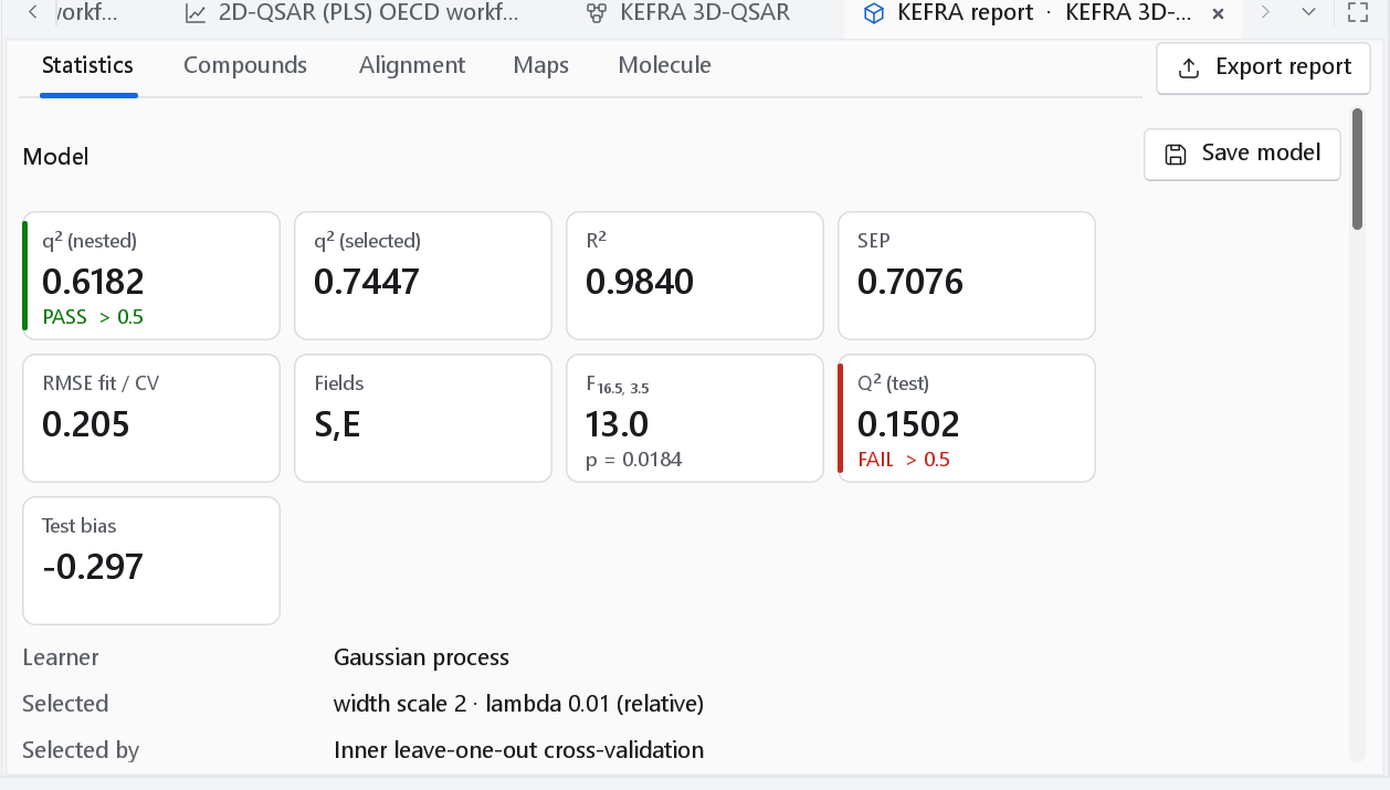
A KEFRA model has no components, so its cards differ:
| Card | Definition | Threshold |
|---|---|---|
| q2 (nested) | Cross-validated q2 with the whole choice of widths and regularisation repeated inside every outer fold (Varma and Simon 2006): no compound influenced the model that predicted it. The number to quote. | Above 0.5 |
| q2 (selected) | The inner leave-one-out q2 at the settings it chose. Biased upwards by that choice; shown for comparison. | |
| R2 | 1 - RSS / SS on the training set. | |
| SEP | sqrt(PRESS / n) of the nested cross-validation. | |
| RMSE fit / CV | The training RMSE divided by the cross-validated RMSE. Far below 1 means the fit is much better than the predictions: the model memorises its training compounds. | |
| Fields | The properties in the fitted kernel. | |
| F | Fisher F of the fit with the effective degrees of freedom of the kernel model, the trace of its hat matrix (Hastie and Tibshirani 1990). The widths and the regularisation were chosen on the same compounds, so its p-value is optimistic. None is reported for kernel PLS. | |
| Q2 (test), Test bias | Q2F1 of the test set, and the mean of observed minus predicted over the test compounds. | Above 0.5 for Q2 |
Below the cards the model summary names the component rule and the cross-validation scheme (SAMPLS when the sample-matrix engine was used), or for KEFRA the learner and the nested q2, and what the fields are computed from: for a hydrophobic field Wildman-Crippen atomic contributions or the data field the model was given instead. These rows are there so that a model is not taken for the output of another program, which would give other numbers for the same compounds.
Per-factor statistics and model statistics
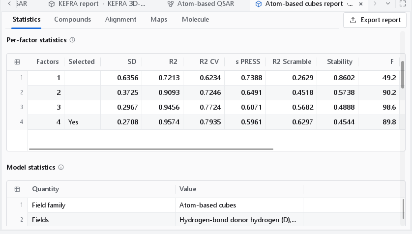
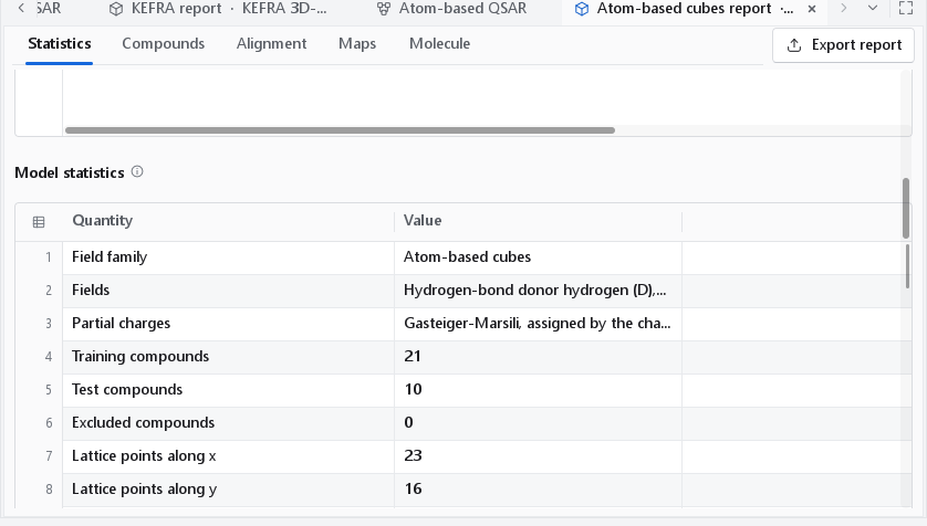
The per-factor table shows how q2 rises and falls with the number of components, which is where over-fitting shows: R2 keeps rising while R2 CV levels off. R2 Scramble is the mean training R2 of the scrambled refits and Stability is RMSE / SEP; both are GeinQSAR definitions. For KEFRA the table lists the settings that were tried and the inner q2 of each. The model statistics list the columns each field kept and its block scale, the cross-validation, the fit, the test set, the field contributions and the resampling runs. Partial charges there names the charge model of the model step itself: when the charges were assigned by a separate step of the preparation, as the builder does for Gasteiger-Marsili charges, it reads As supplied, and the Preparation table of the Alignment tab names the method.
Field contributions gives the share of the model carried by each field or atom class: for the cubes the share of the total |StDev x Coeff|, the usual field fraction of 3D-QSAR.
Repeated cross-validation and cubes
When the model was built with region focusing, the Statistics tab says so in one line: q2 is then not an honest cross-validation and the model has to be judged by its test set. Warnings of the run, such as compounds without an activity, are listed at the end of the tab.
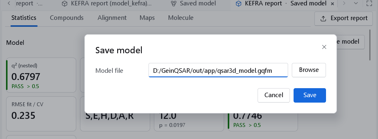
Save model
Save model, on the row of the Model title, writes the model as a .gqfm file, exactly as Save the model of the wizard does.
Documents\GeinQSAR\Output.Compounds
| Column | Meaning |
|---|---|
| Set | Training, Test, or Excluded (no activity, or left out by the set column). |
| Observed | The measured activity. |
| Fitted | The model's value for a training compound. |
| CV predicted | The value of a training compound from the model built without it; the numbers q2 is computed from. |
| Test predicted | The value of a test compound, which took no part in the model. |
| Beyond lattice (Å) | Atom-based cubes: how far the atoms of the compound reach outside the lattice. A compound that reaches beyond it has part of itself sampled nowhere, so its prediction is an extrapolation; the tab counts such compounds. Not shown for KEFRA, which has no lattice. |
The observed against predicted chart is below the table. Rows selected in the table are highlighted in the chart, and a brush in the chart selects rows; Clear selection empties both. The camera button of the chart opens the figure dialog.
Alignment
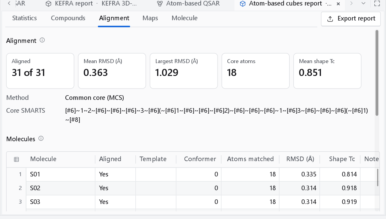
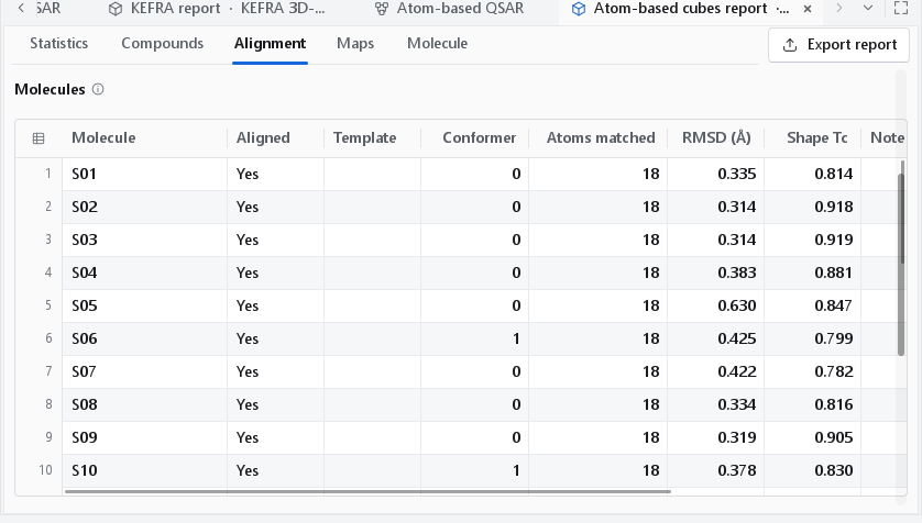
Both models compare the molecules in the frame of the alignment, so this tab is where a weak model is diagnosed first: one molecule with a large RMSD or a low shape Tanimoto spoils the model.
| Column | Meaning |
|---|---|
| Aligned | Whether the molecule could be placed. |
| Template | Marks the molecule every other one was superposed onto. |
| Conformer | The stored conformer that was superposed, counted from 0 (the lowest in energy). |
| Atoms matched | The atoms the fit of the molecule rests on. |
| RMSD (Å) | Their deviation after the fit. Empty for a method that matches no atoms (As supplied, shape, inertial frame). |
| Shape Tc | Gaussian shape Tanimoto with the template (Grant and Pickup 1995). |
| Note | Why a molecule could not be placed, or how it was placed when not by the common core. |
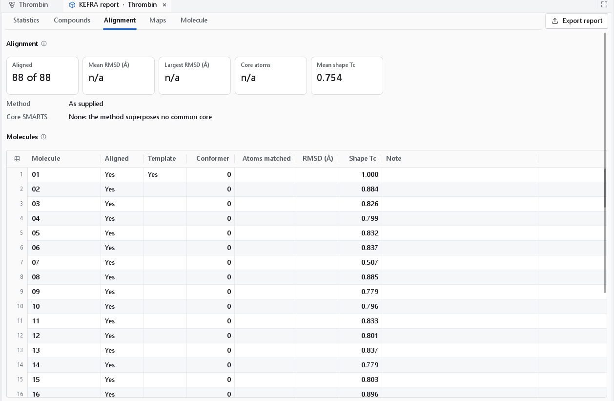
Below the molecules, Preparation lists every step the compounds of the model went through (standardisation, embedding, conformers, charges, alignment) with every parameter. That table is what the prediction wizard replays for new compounds.
Maps
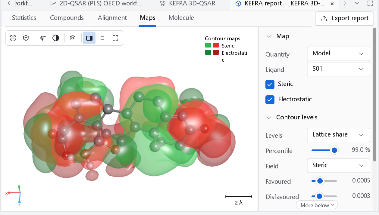
The Maps tab draws the model as a 3D map with one compound inside it for orientation. How to read the maps, what the colours and levels mean, and every control of the panel are on Contour maps and atom cubes.
Molecule
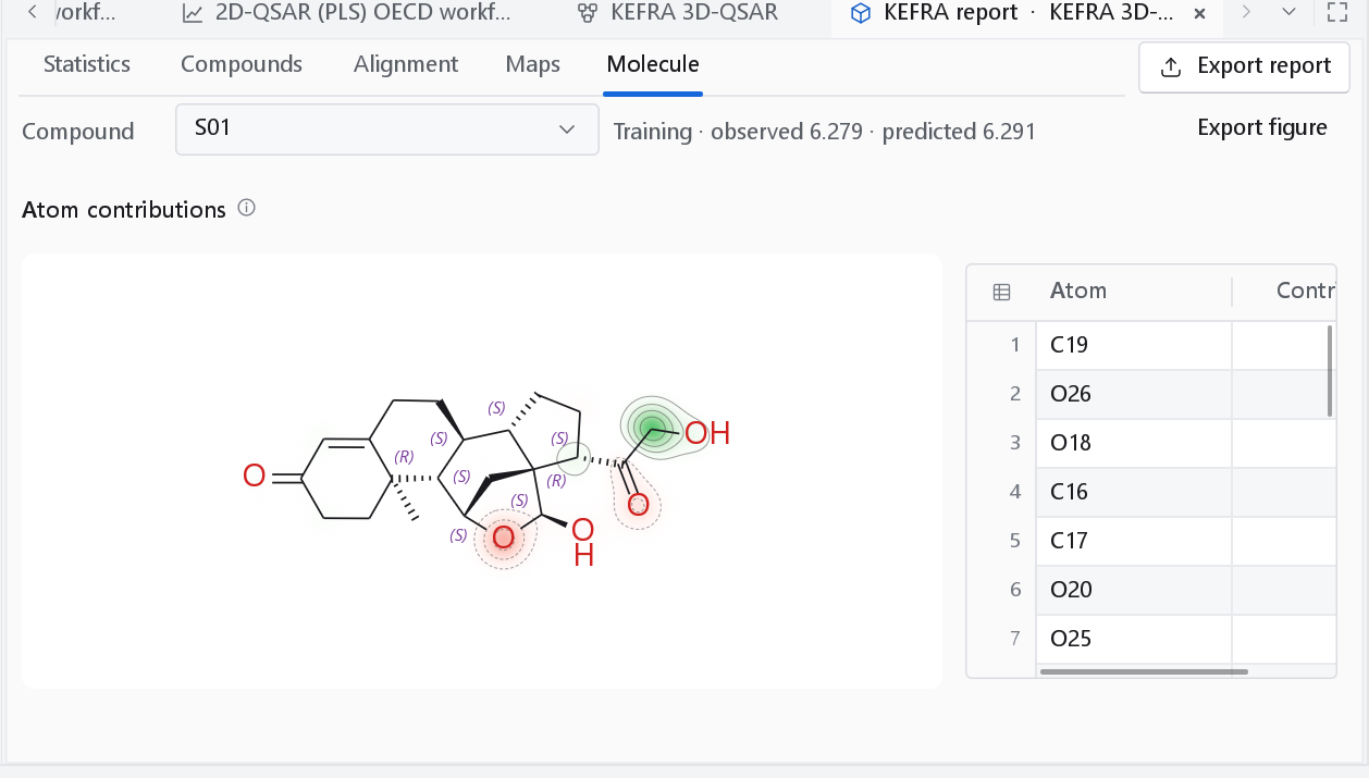
Choose the compound in Compound. The line next to it gives its set and its observed and predicted values. The contribution of each region of space to the prediction is assigned to the atoms near it, so the 2D drawing shows which parts of the molecule the model credits and blames. Export figure writes the coloured compound as an SVG figure.
Opening a saved model
File > Open on a .gqfm file, or the file dropped on the window, opens a small workflow that reads it and this dashboard with the same statistics, compounds and maps. The tab is named after the file. Nothing is recomputed: the file holds the fitted model.
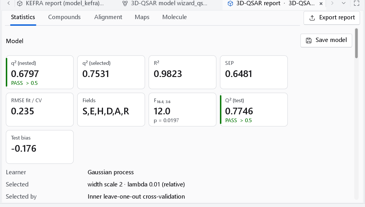
.gqfm file: the same cards as the run that saved it, here a model with four test compounds and a test-set Q2 of 0.9760.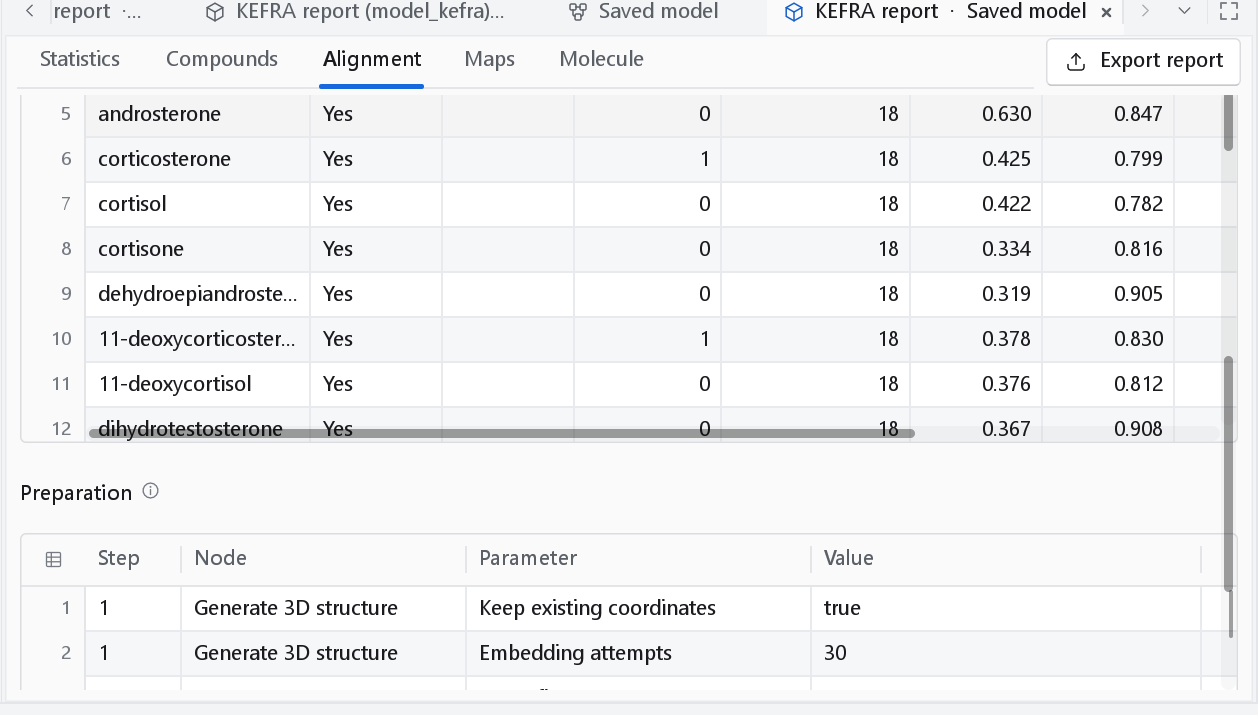
The Alignment tab of a saved model has no alignment report, because the file holds the aligned compounds and the record of their alignment, not the report of the alignment run; it does have the Preparation table. The model can be applied to new compounds with Wizards > Predict with a saved model (see Predicting new compounds).
Export report
Export report writes the report of the model as a PDF, a Word document and an Excel workbook, in whichever of the three you tick, with the statistics, the figures, the predictions and, when the workflow is still open, the workflow itself, so that the report can be reproduced. Tables as CSV also writes the per-factor statistics, the field contributions, the model statistics, the per-compound predictions, the alignment report and the contour levels as CSV files. See Reports and export.
The report carries two residual figures that the dashboard does not draw: the residuals against the observed activity, with the band at 2.5 standard deviations marked, and the distribution of the residuals of each set side by side. Read them together with the bias on the Statistics tab. What they are for is to show that the errors have no mean and no trend, which a single Q2 cannot show, and to name the compounds the model gets wrong instead of leaving them inside an average.