The model dashboard
The report of a regression model: the acceptance criteria, the validation figures, the descriptors, the applicability domain and every prediction, read from the run that built it.
The model dashboard opens when a regression workflow finishes, whether the workflow came from the 2D-QSAR wizard, a template or the canvas. It does not compute anything of its own. Every number and every figure is read from the output of the validation node of the workflow, so the dashboard, the exported report and the files the workflow wrote always agree. A workflow that validates several models side by side opens one dashboard per model, with the primary model in front.
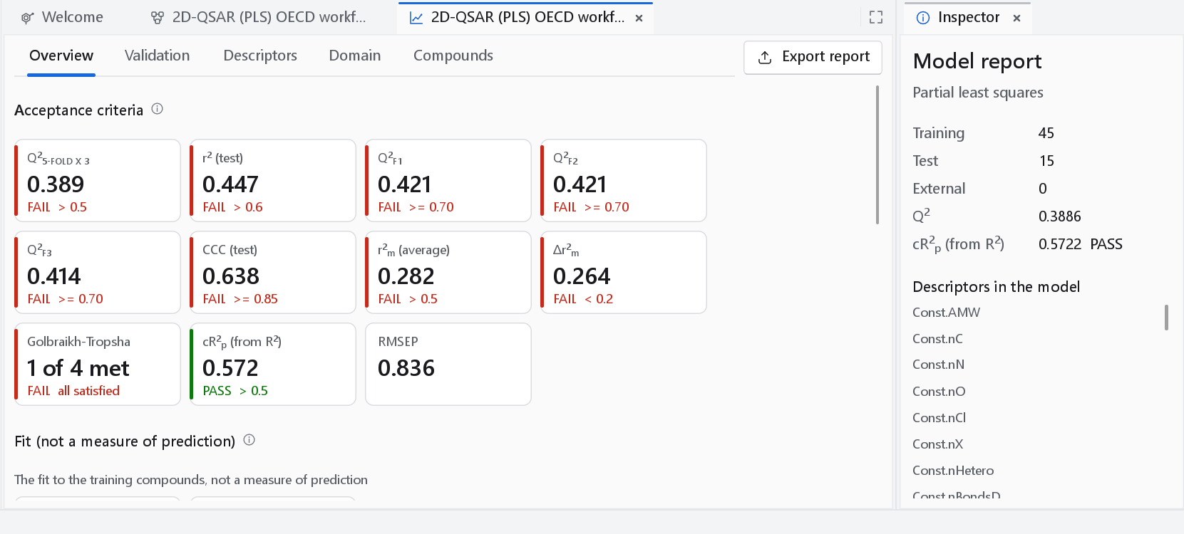
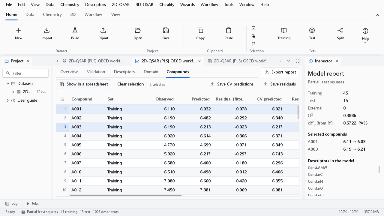
The dashboard has five tabs: Overview, Validation, Descriptors, Domain and Compounds. Export report at the right of the tab bar writes the report of the run as PDF, Word or Excel (see Reports and export). The inspector on the right summarises the model: its type, the number of training, test and external compounds, Q2, the Y-randomisation statistic with its verdict, the compounds you have selected with their observed and predicted values, and the descriptors the model uses.
| Control | What it does |
|---|---|
| Card | One statistic. A card with an acceptance threshold shows the threshold and a PASS or FAIL badge, and a coloured bar on its left edge: green for a pass, red for a fail. |
| Help mark | The small circled i next to a heading. Its tooltip explains the section and, for a figure, what the run says about it (the space the leverage was computed in, the value of h*). |
| Camera button | At the right of every chart. Opens the figure dialog for that chart (see Publication figures). |
| Save as CSV | At the right of a table heading. Writes the table as the run produced it, at full precision. |
| Tooltip of a card | The definition of the statistic and the reference its threshold comes from. |
Overview: the acceptance criteria
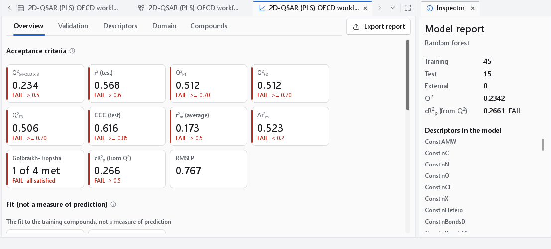
The first section, Acceptance criteria, is one card per statistic of the published validation criteria for regression QSAR models. A criterion that fails is reported as measured; the dashboard does not hide or soften it. Read the cards in three groups: goodness of fit (R2 of the training set), robustness (the cross-validated Q2 and the Y-randomisation statistic) and predictivity (everything computed on the test set). A model is judged on the last two groups. The training R2 has no threshold because a flexible model can always raise it.
| Card | What it measures | Accepted when | Reference |
|---|---|---|---|
| R2 (training) | 1 - SS(residual) / SS(total) on the training compounds. Goodness of fit only. | no threshold | Draper and Smith, Applied Regression Analysis, 3rd ed., Wiley 1998 |
| Q2 with the scheme as subscript (for example 5-FOLD X 3) | 1 - PRESS / SS(total), each training compound predicted by a model fitted without it. The subscript names the cross-validation scheme and the repeats. | > 0.5 | Golbraikh and Tropsha, J. Mol. Graph. Model. 20:269 (2002) |
| R2 (test) | R2 of the test compounds, which took no part in the model. | > 0.6 | Golbraikh and Tropsha (2002) |
| Q2F1 | 1 - PRESS(test) / SS of the test values about the training mean. Punishes a test set whose mean differs from the training mean. | >= 0.70 | Shi et al., J. Chem. Inf. Comput. Sci. 41:186 (2001); threshold: Chirico and Gramatica, J. Chem. Inf. Model. 52:2044 (2012) |
| Q2F2 | 1 - PRESS(test) / SS of the test values about their own mean. | >= 0.70 | Schüürmann et al., J. Chem. Inf. Model. 48:2140 (2008) |
| Q2F3 | 1 - [PRESS(test) / n(test)] / [SS(training) / n(training)]: the test error scaled by the spread of the training set, so it does not depend on how the test values happen to be distributed. | >= 0.70 | Consonni, Ballabio and Todeschini, J. Chem. Inf. Model. 49:1669 (2009) |
| CCC (test) | Concordance correlation coefficient: how closely the observed and predicted test values lie on the identity line, not merely on some line. | >= 0.85 | Lin, Biometrics 45:255 (1989); Chirico and Gramatica (2011, 2012) |
| r2m (average) | Mean of r2m and r'2m, where r2m = r2 (1 - sqrt(r2 - r02)) with r02 from the regression through the origin. | > 0.5 | Roy et al., J. Chem. Inf. Model. 52:396 (2012) |
| Δr2m | Absolute difference of r2m and r'2m for the two axis assignments. A large value says the predictions are biased in scale. | < 0.2 | Roy et al. (2012) |
| Golbraikh-Tropsha | Counts how many of the individual test-set conditions are met: R2(test) > 0.6, a slope k or k' of the regression through the origin between 0.85 and 1.15, and (R2 - R02) / R2 < 0.1. | all satisfied | Golbraikh and Tropsha (2002) |
| cR2p (from R2) or (from Q2) | R sqrt(R2 - mean R2 of the Y-randomised models), or the same with the cross-validated Q2. A chance correlation gives a value near 0. | > 0.5 | Mitra, Saha and Roy, Mol. Simul. 36:1067 (2010) |
| RMSEP | Root mean squared error of the test predictions, in the units of the response. The number to quote as the expected error of a prediction. | no threshold | Draper and Smith (1998) |
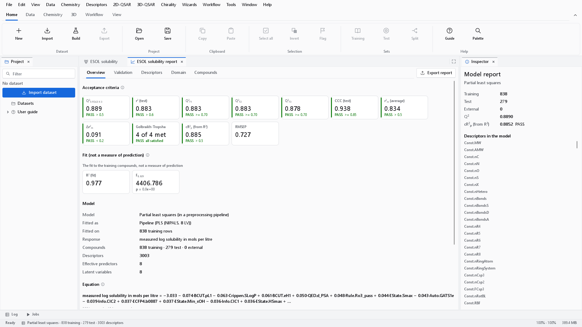
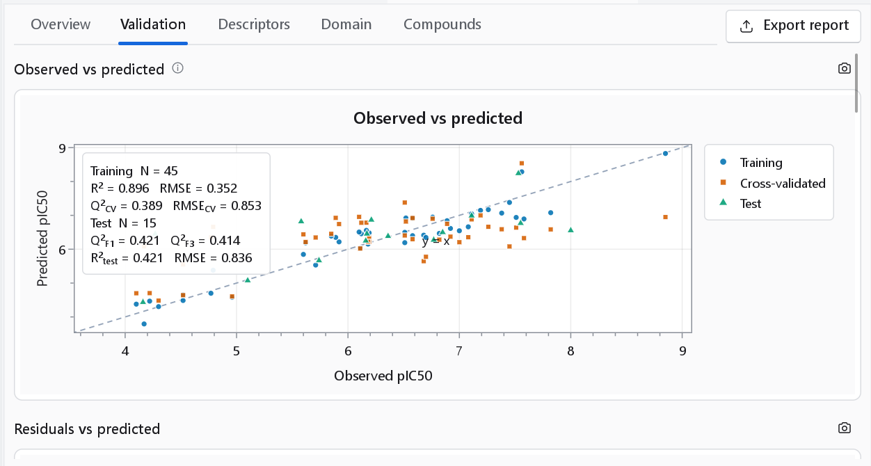
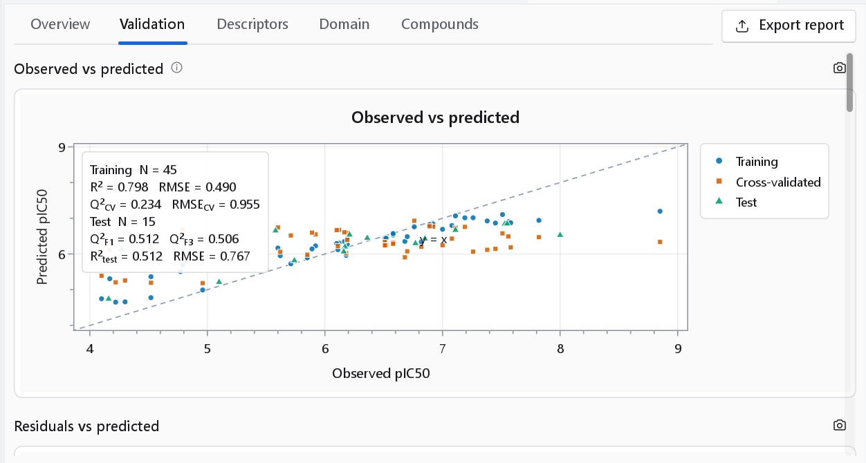
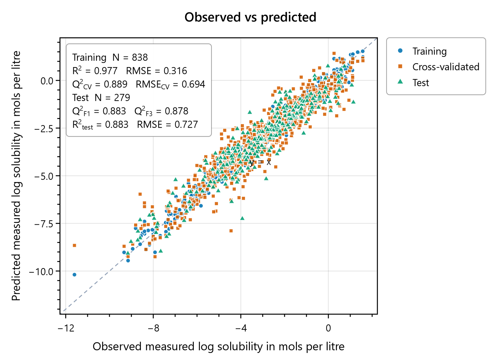
What a passing model looks like: the ESOL aqueous solubility set (1128 compounds, 838 training and 279 test, the default recipe with three repeats of 5-fold cross-validation) gives R2 0.977, Q2 0.889, R2 (test) 0.883 and RMSEP 0.727 log units, and passes every card. The PLS model on 60 acetylcholinesterase inhibitors above, with about a thousand descriptor columns, fails nearly all of them. The difference is the data, not the program: 45 training compounds do not support a model on a thousand descriptor columns.
Model, equation and All metrics
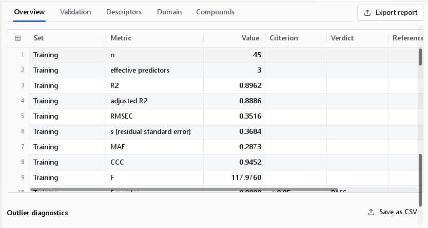
Under the cards, Model lists what was fitted: the model type, Fitted as (the pipeline with its preprocessing and, for PLS, the number of latent variables), Fitted on (how many training rows), the response, the compounds per set, the number of descriptors, the effective predictors and the latent variables. A linear model also shows its Equation; when it has more terms than fit on the page, the largest are shown and a line says how many there are. The warnings of the run follow, then All metrics: every statistic the validation produced, including those without a card, with the set it belongs to, its value, the criterion, the verdict and the reference. Counts are printed as integers (n = 45) and the Golbraikh-Tropsha row as yes or no. A statistic that could not be computed is left empty, never shown as zero.
Validation
The Validation tab shows every figure the validation node delivered, each under the title the run gave it, and nothing the run did not produce. A figure that is absent takes no place and prints no heading.
| Figure | What to look for |
|---|---|
| Observed vs predicted | Training, cross-validated and test predictions as three series against the identity line, with a statistics box (N, R2, RMSE, Q2CV, Q2F1, Q2F3, R2test). The cross-validated points are the honest ones for the training compounds; a cloud of training points tight on the line with the cross-validated points spread around it is the picture of overfitting. |
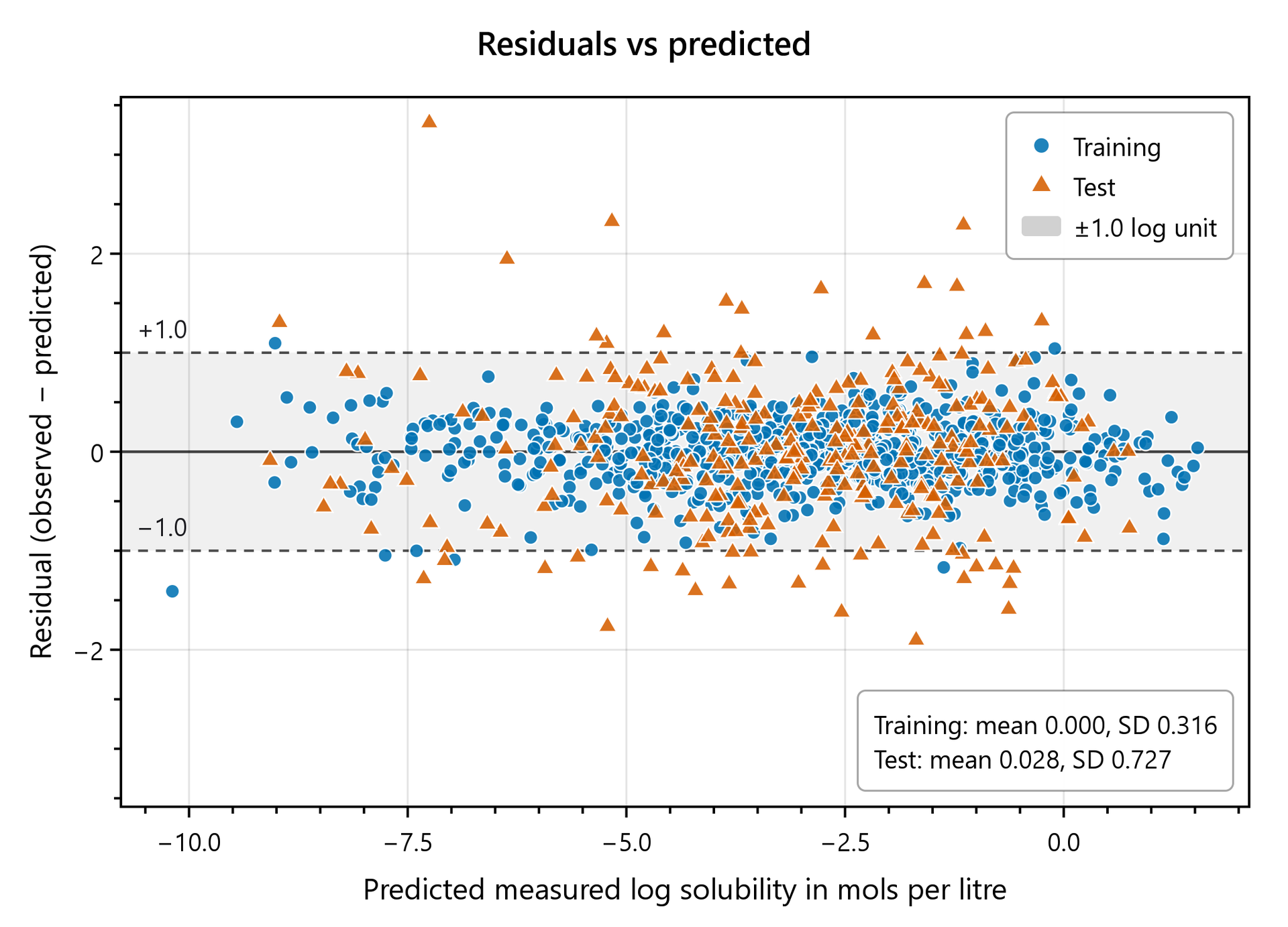
| Residuals vs predicted | Observed minus predicted against the prediction, with a band of one log unit. A funnel says the error depends on the activity range. A downward trend is expected for every compound the model did not fit, where the slope of the residual on the prediction is about minus var(residual) / var(predicted); the trend itself is read from the residual slope rows of All metrics, which carry that expected value beside the measured one. On the training compounds the same slope measures only how far the fit was shrunk towards the mean: it is exactly zero for least squares and PLS, and positive for ridge, kernel and forest models. All metrics reports it there without an expected value and without a p-value, because it cannot show a fault. |
| Williams plot, or its replacement | See Domain below. For a model without a hat matrix the figure is the standardised residual against the distance the domain measures, and it is titled accordingly. |
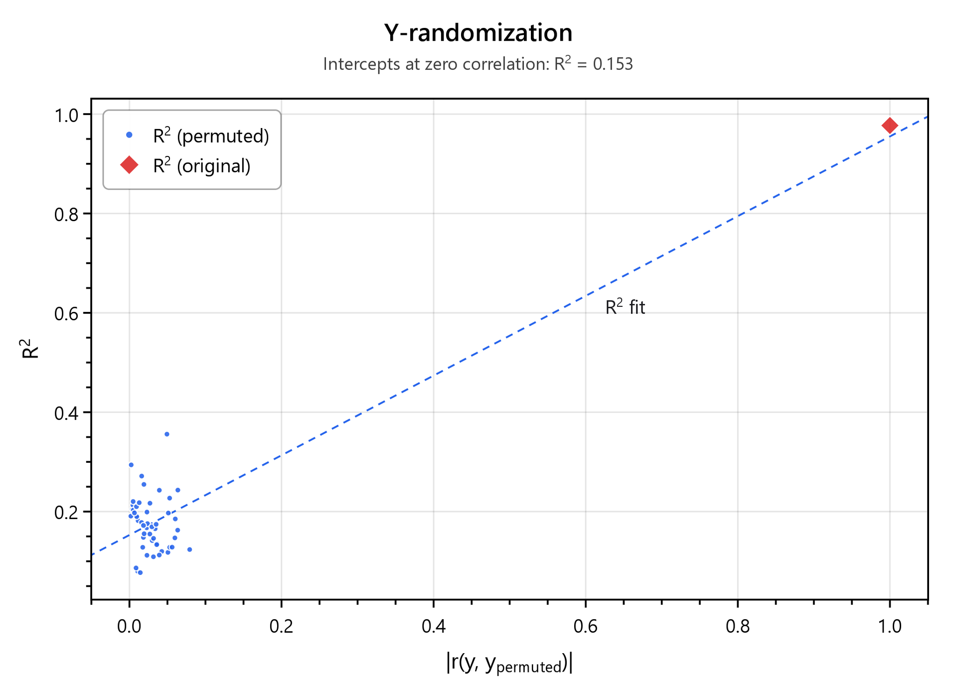
| Y-randomisation | One point per permuted model: its R2 (and Q2 when computed) against the correlation of the permuted with the true response, and the true model at correlation 1. The permuted points should sit far below the true one. |
Y-randomisation: which statistic decided
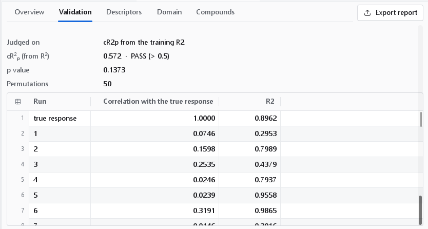
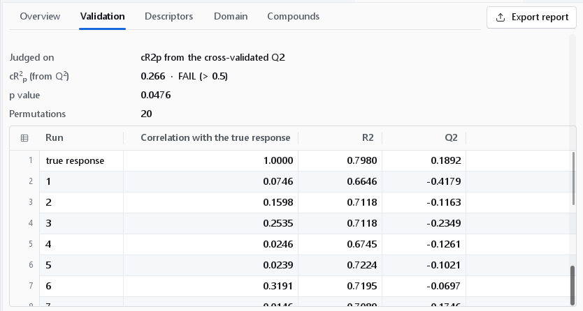
Below the figures the Y-randomization section says on which statistic the verdict was judged (Judged on), its value and verdict, the p value of the permutation test, the number of Permutations and a table with the true model in its first row and one row per permuted run: the correlation of the permuted with the true response, R2 and, when computed, Q2.
| Judged on | Statistic | Used for |
|---|---|---|
| cR2p from the training R2 | R sqrt(R2 - mean R2 of the permuted models), on the training rows | MLR, stepwise MLR, PLS, PCR, ridge and elastic net |
| cR2p from the cross-validated Q2 | Q sqrt(Q2 - mean Q2 of the permuted models), cross-validated on the same folds as the model | every other model type |
A random forest or a support vector machine reproduces scrambled activities on its own training rows, so its training R2 is no evidence against chance correlation; the cross-validated form is. The 0.5 limit was proposed for the training-R2 form and is carried over to the cross-validated one (Rücker, Rücker and Meringer, J. Chem. Inf. Model. 47:2345, 2007, for the method). Read the p value together with the card: it is the share of permutations that scored at least as well as the true model.
Descriptors
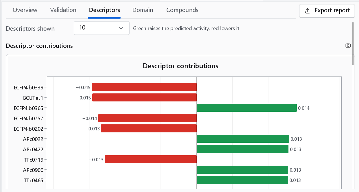
The Descriptors tab shows the Regression coefficients of a linear model, the VIP scores of a PLS model (variable importance in the projection: descriptors with VIP above 1 carry more than their share of the model), the correlation matrix of the model descriptors and a PCA of the descriptor space. These are the mechanistic-interpretation part of the OECD principles.
Domain
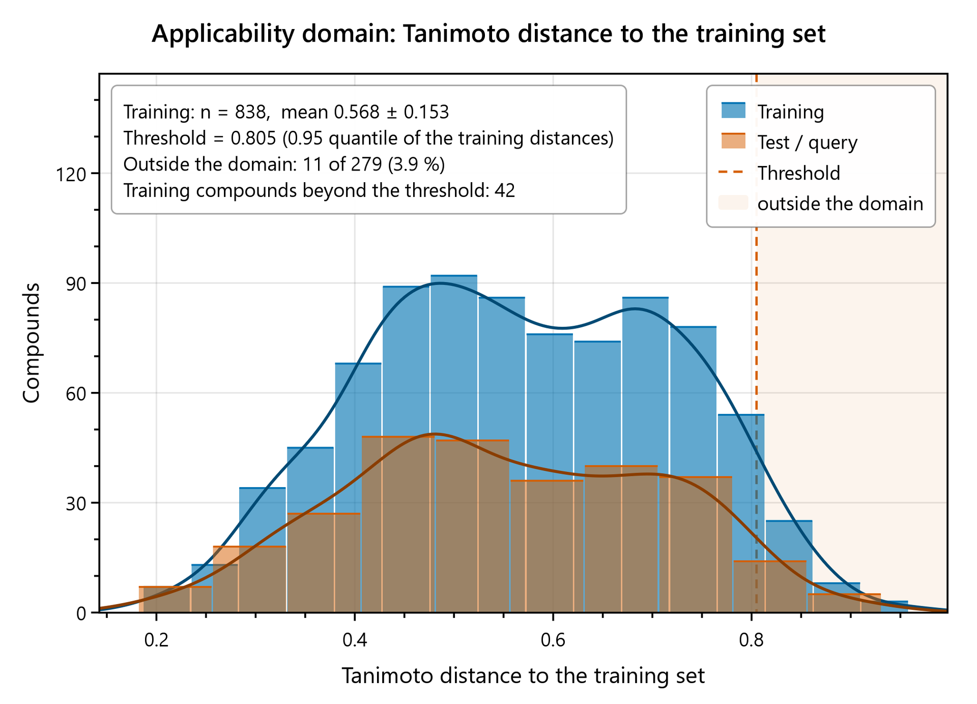
The applicability domain is the region of descriptor space the training set covers; a prediction outside it is an extrapolation. The domain is fitted on the training compounds together with the model and stored with it, so the verdicts shown here are the ones a later prediction gives.
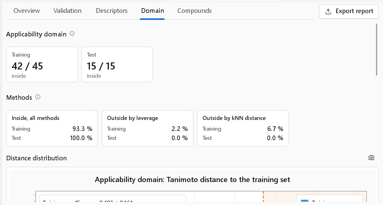
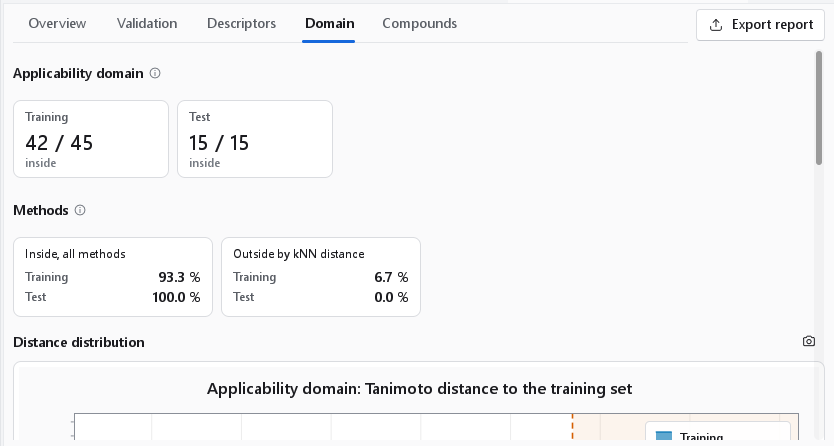
- Applicability domain: one card per set, the number of compounds inside out of the set (42 / 45, 15 / 15).
- Methods: a card for the combined verdict (Inside, all methods, as a share of each set) and one card per method that was fitted (Outside by leverage, Outside by kNN distance) with the share of each set that this method alone places outside. The tooltip of a card gives its threshold.
- Distance distribution: the histogram of the distance the domain measured, for the training compounds and for the others, with the threshold as a dashed line. Its axis names the space (the distance over the model columns, or the Tanimoto distance over the fingerprint columns) and its statistics box states the threshold with the rule that produced it.
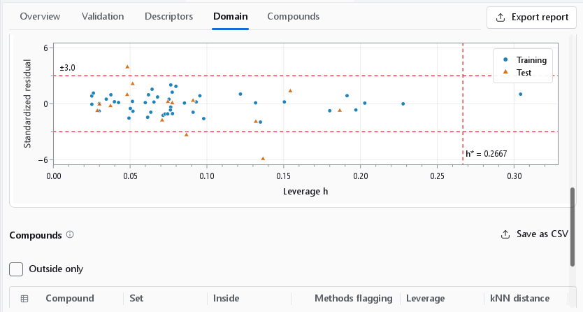
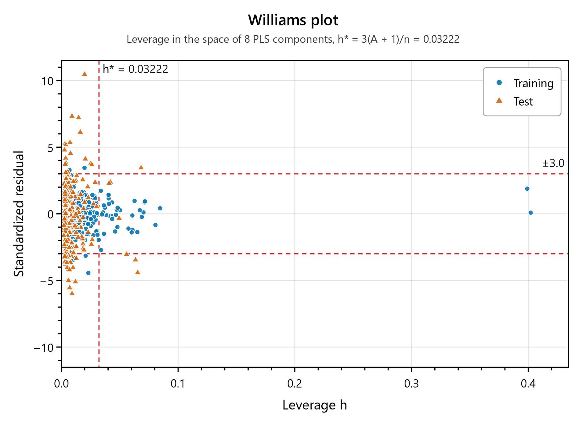
- The domain figure of the run under its own title: the Williams plot, or for a model without a hat matrix the residual against the distance to the training set.
- Compounds: one row per compound with the set, the combined verdict (Inside), the number of Methods flagging it and one column per method. Outside only keeps the compounds the combined rule places outside; Save as CSV writes the table.
| Method | Definition | Reference |
|---|---|---|
| Leverage | h = x'(X'X)-1x in the regression space of the model, with the warning leverage h* = 3 (A + 1) / n: A latent components of a PLS or PCR model (or the descriptors of an MLR model) and n training compounds. | Gramatica, QSAR Comb. Sci. 26:694 (2007) |
| Williams plot | Standardised residual against leverage. A compound with a residual beyond ±3 is a response outlier; one beyond h* is a structural outlier, predicted by extrapolation. | Eriksson et al., Environ. Health Perspect. 111:1361 (2003) |
| kNN distance | Mean distance to the 5 nearest training compounds. The threshold is set from the same distances inside the training set; the default is their 0.95 quantile, and the statistics box of the distance distribution names the rule that was used. | Tropsha, Gramatica and Gombar, QSAR Comb. Sci. 22:69 (2003); Sahigara et al., Molecules 17:4791 (2012) |
| Descriptor range, PCA bounding box | Inside the range the training set spans in every descriptor, or in every principal component. Off by default. | Sahigara et al. (2012) |
| DModX, Hotelling T2 | Distance to the model and distance inside the score space of a latent-variable model, each with its F-based critical value. Off by default. | Eriksson et al., Multi- and Megavariate Data Analysis, Umetrics 2006 |
By default a compound is outside when the leverage or the kNN distance flags it. The rule is set in the wizard (Outside the domain when, see The 2D-QSAR wizard).
Compounds and the linked spreadsheet
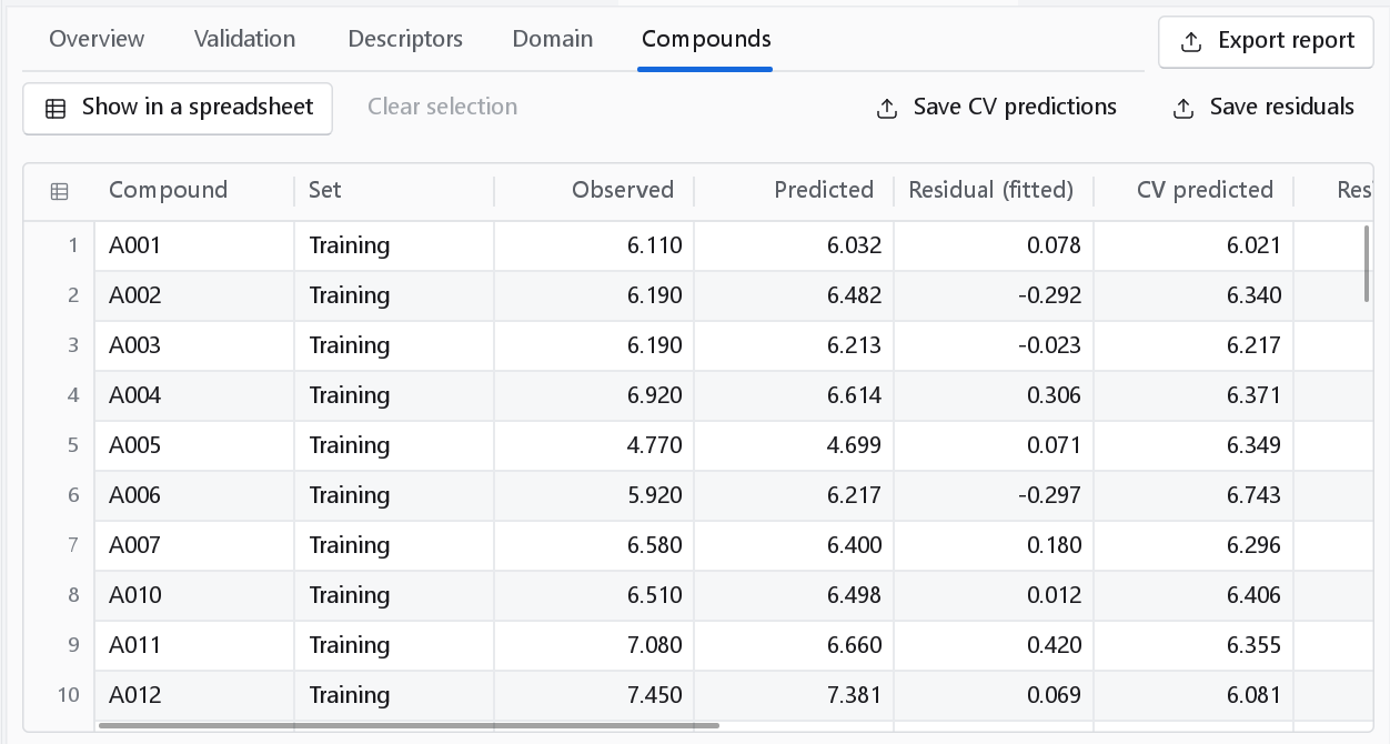
The Compounds tab lists every prediction: compound, set, observed, predicted and residual, the cross-validated prediction with its residual and how often the compound was held out, and the domain flag. Save CV predictions writes the cross-validated predictions, the numbers Q2 is computed from.
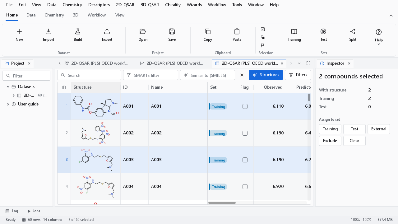
The compound table and the scatter plots of the dashboard share one selection: select points in a plot and the rows are selected, and the other way round. A permuted model in the Y-randomisation figure selects nothing, because it is not a compound. Show in a spreadsheet opens the predictions as a dataset with structures that shares the same selection; Clear selection empties it.
Where the numbers come from
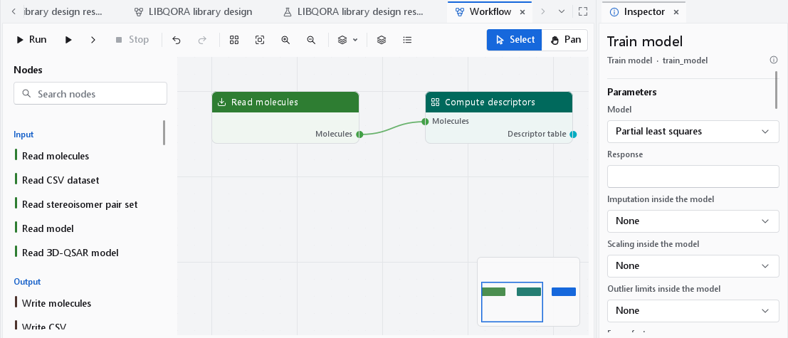
A dashboard belongs to the workflow that produced it. The model type, its hyper-parameters, the preprocessing inside the model and the domain settings are parameters of the Train model node; select the node on the canvas and the inspector shows them. Change one and run the workflow again to get a new dashboard; Workflow > Open results dashboards reopens the dashboards of the last run.
Figures for a paper
The camera button of a chart opens the figure dialog: SVG or PNG, the size in millimetres or pixels, the resolution, and Publication figure (170 mm, 600 dpi, the publication theme) in one step. Below 120 mm, a single-column figure, the chart is adapted to the width: smaller text, closer ticks, no statistics box (its numbers belong in the caption) and the legend beside the frame. The figures of this page marked as print figures were written this way at 174 mm and 300 dpi. See Publication figures for every option.