A tour of the software
What each part of the window is for, how the numbered workflow on the left drives a docking study, and how the panels around the viewer report on it.
The window is arranged around one idea: the docking workflow runs top to bottom down the left hand side, and everything else in the window either feeds it or explains its results. Once you can see that, the rest of the application follows.
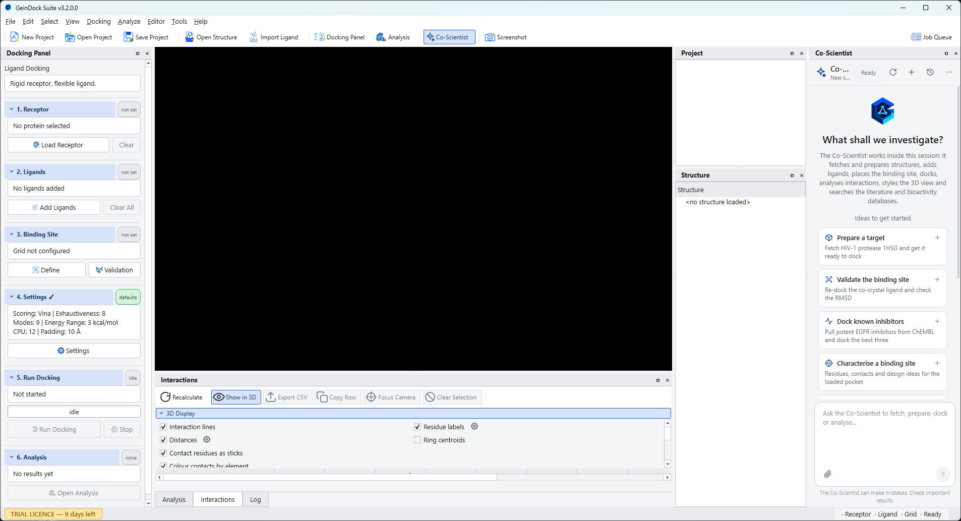
The five regions of the window
| Region | What it is for |
|---|---|
| Menu bar | Every command the application has, grouped by subject. Commands that need something you have not loaded yet are greyed out rather than hidden, so you can see what will become available. |
| Toolbar | The commands used most often, in groups from left to right: New Project, Open Project and Save Project; Open Structure and Import Ligand; Docking Panel and Analysis; Co-Scientist, which shows or hides the assistant; and Screenshot. Job Queue sits on its own at the far right, because it opens a separate window rather than a panel. |
| Docking Panel | The numbered workflow, on the left. Six steps, each with a chip telling you whether it is done. This is where a docking study is actually driven. |
| 3D viewer | The centre of the window. Everything you load or compute is drawn here, and it is a full molecular viewer rather than a preview: you can select, measure, restyle and export from it. |
| Dockable panels | Project, Structure, Co-Scientist, Analysis, Interactions and Log. Each can be moved, floated, tabbed with another or closed, and the arrangement is remembered between sessions. The Job Queue is the exception: it is a separate floating window that you open, glance at and close, and it cannot be docked into the main window. |
The Docking Panel
The panel on the left is the spine of the application. It has six numbered steps, and a heading above them naming the docking mode that is currently active.
| Step | What it asks of you |
|---|---|
| 1. Receptor | The protein you are docking into, cleaned and protonated. |
| 2. Ligands | One or more compounds to dock, in three dimensions and ready for the search. |
| 3. Binding Site | Where on the protein to look, expressed as a box. |
| 4. Settings | How hard to search, and with which scoring function. In the three specialised modes this step changes into the picker that mode needs instead. |
| 5. Run Docking | Start the job, watch it, and stop it if you need to. |
| 6. Analysis | Open the pose table once results exist. |
Every step carries a small chip on the right of its heading that tells you its state at a glance: not set when nothing has been supplied, loaded or added when something is there but is not yet ready to dock, and prepared or configured when the step is complete. A tick also appears beside the step number when it is done. The Run Docking button stays disabled until every step it depends on is green, and hovering over it tells you which one is missing.
The panels around the viewer
Project
Lists everything loaded in the current session, including the receptor, the ligands and each complex a docking run produced. Selecting an entry brings it to the front of the viewer.
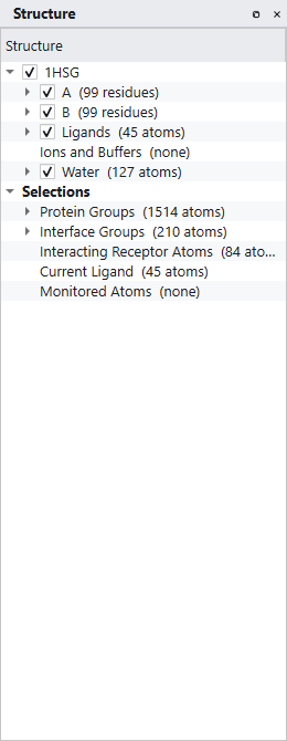
Structure
A tree of everything in the scene, broken down by model, chain, residue and atom, with separate branches for ligands, ions and buffers, and water. Every branch has a checkbox that shows and hides it, and a right click menu that restyles, recolours or selects what is under the cursor. Below the structure branches sit the selection groups, which is where you find the interface residues, the interacting receptor atoms and the current ligand.
Analysis
The pose table. Empty until a run finishes, then filled with one row per ligand, expandable to one row per pose. This panel also carries the Interactions and Log tabs.
Interactions
The contacts between the receptor and whichever pose is selected, listed by type, distance and geometry, with a Show in 3D toggle that draws them in the viewer.
Job Queue
A window of its own rather than a panel, opened with the Job Queue button at the far right of the toolbar. It floats over the main window, can be moved and closed, and cannot be docked or tabbed with the panels. One row per job, expandable into the steps that make it up, with the state, the result, a progress bar, a detail column and an elapsed clock. Jobs survive in this list after they finish so you can compare them.
Log
The running commentary from the application and from the backend. When something goes wrong, this is the first place to look.
Co-Scientist
The research assistant, in a full height column at the right hand edge of the window, beside Project and Structure. Type a request at the bottom of the panel and it works on the session you have open, recording each operation in the conversation as it goes. The Co-Scientist button on the toolbar shows and hides the panel, as does View › Panels › Co-Scientist. It is the one panel that needs an internet connection. See Meet the Co-Scientist.
A first look at a structure
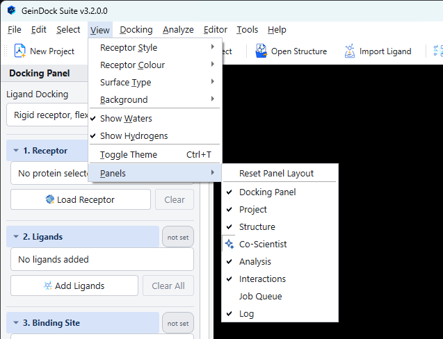
You do not have to start a docking study to try the viewer. File › Open Structure loads any structure file into the scene, and from there the whole of View becomes live: ten representations, eighteen colouring schemes, four surface types and a choice of backgrounds.
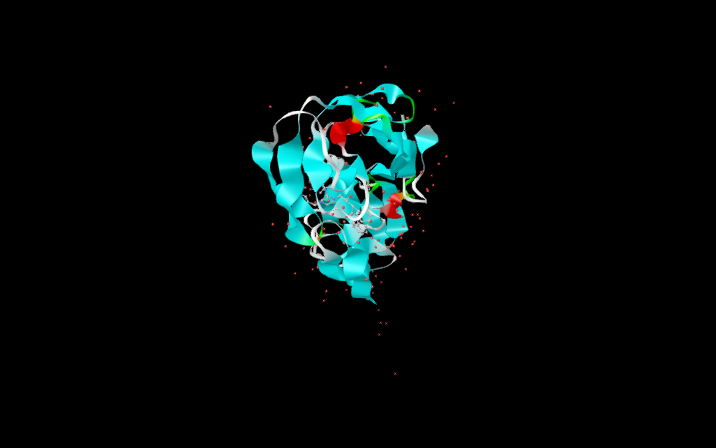
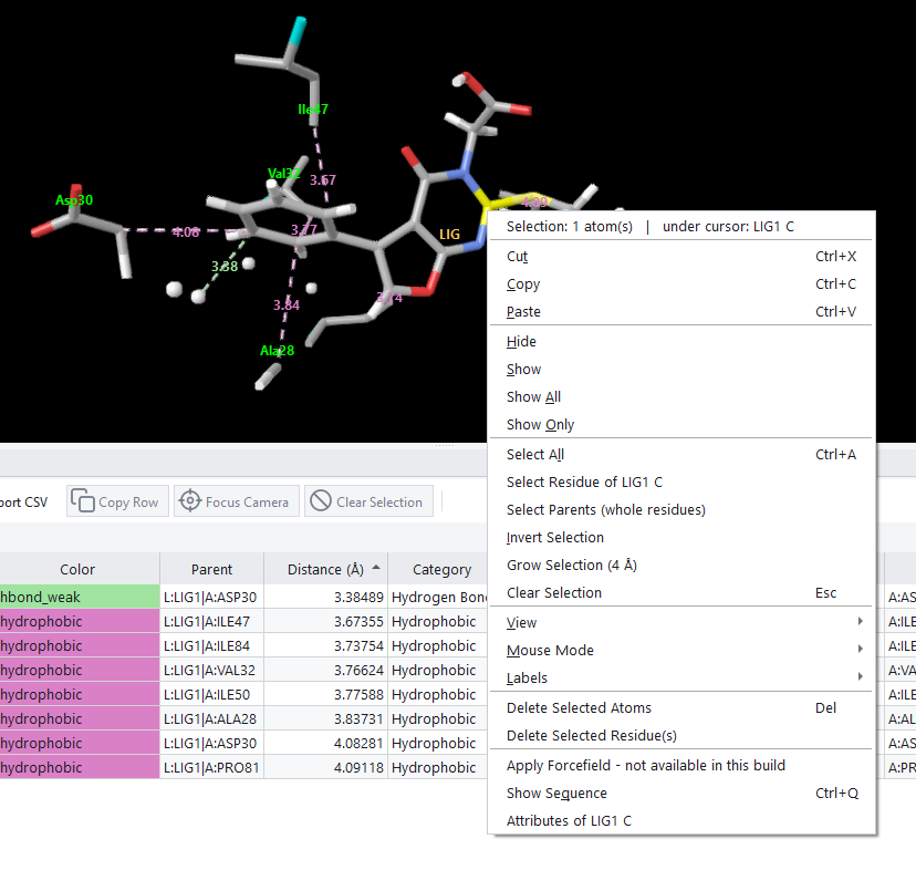
The mouse works the way it does in every molecular viewer: drag with the left button to rotate, drag with the middle button to pan, and roll the wheel to zoom. Right clicking anywhere in the viewport opens a context menu that names what is under the cursor and offers the selection, visibility and view commands that apply to it.
Where to go next
If you want to run a docking job now, go to The Docking Panel and follow it from step 1. If you would rather understand the choices first, read Which mode do I need?, which explains what the four docking protocols are for and what each one asks you to supply. If you would like the software to take the first steps for you while you watch, read Meet the Co-Scientist.