The Results page
Opening finished jobs, reading the overview and the figures, switching units, computing missing analyses, and opening several results side by side.
The Results page is where a finished job is read. It lists every analysis the job has, draws each one as the same figure that the exported report and image files carry, and puts the numbers behind the figure in a table beside it. Nothing on the page is a separate rendering: the figure on the screen is byte for byte the image the export writes, so what you check here is what a reader of the report will see.
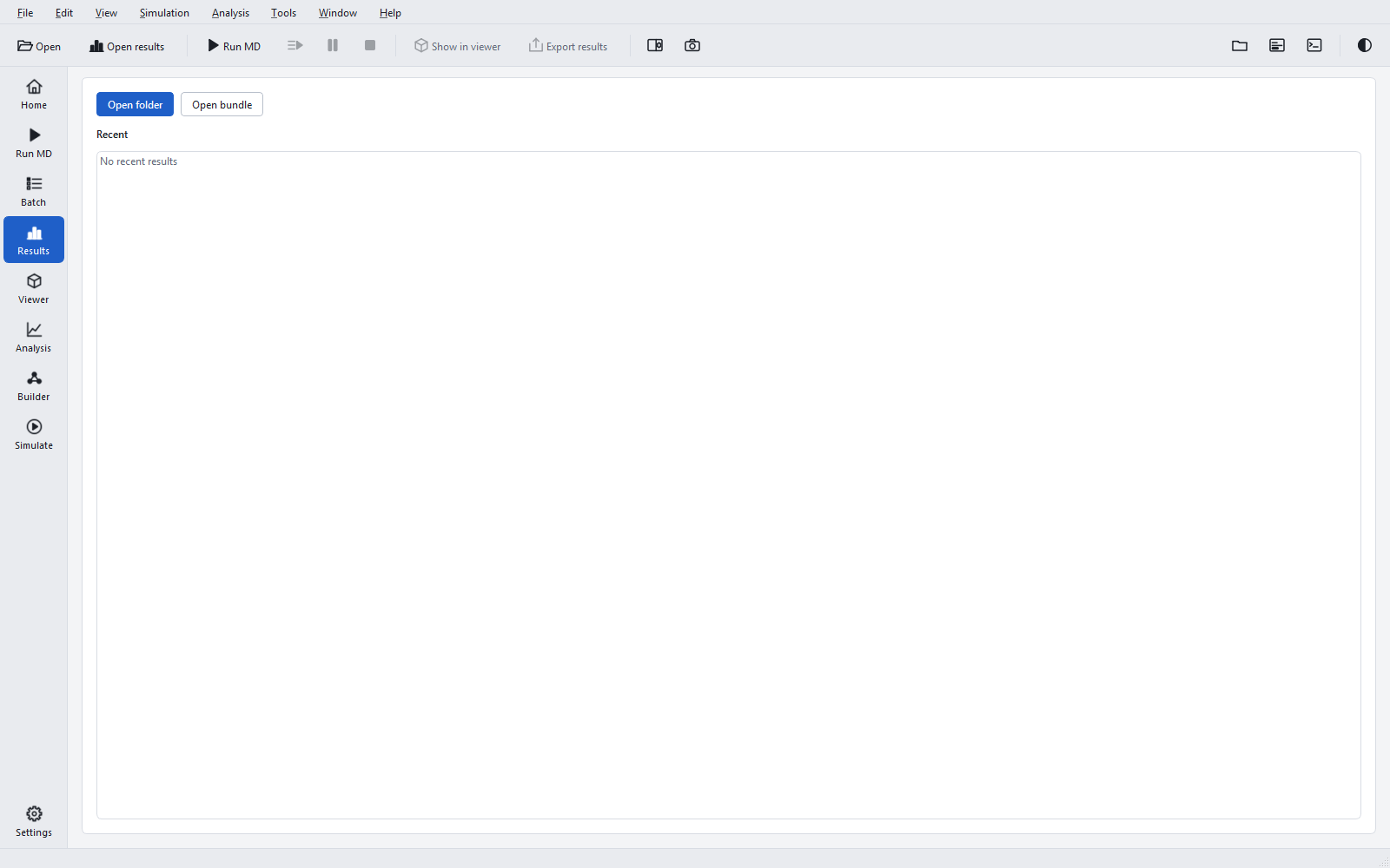
Opening results
| Route | What it opens | When to use it |
|---|---|---|
| Open folder on the start screen, or File > Open results folder (Ctrl+Shift+O) | The folder of a finished job, or a folder that contains several job folders. A folder of jobs is opened as a batch: every job appears in the compound selector and the Comparison group is added to the navigation. | The usual route for a job on this PC. |
Open bundle, File > Open result bundle (.gnm), drag and drop, or Geinium.exe file.gnm | A result bundle: one file that holds a complete job without its checkpoints and raw trajectories (see Result bundles at the end of this page). | Results that were made on another PC or are to be archived. |
| Recent | Any result opened before, by a double-click. | Going back to a job you looked at recently. |
| Results on the Run MD page, the Batch page or the Jobs panel | The job that has just finished. | Straight after a run. |
| Add results in the header | Another job beside the open one. | Comparing compounds; see Comparing compounds. |
The page is also reached with Ctrl+4 or the Results button of the page bar. The status bar names the number of trajectory frames and the time span of the open job.
The header
The bar above the navigation belongs to the open job. From left to right: the job name (a drop-down list when several jobs are open), Add results, three fact chips (number of atoms, production length times the number of replicas, for example "100 ns × 1", and the speed of the production run in ns/day), the two unit choices, Show in viewer, Export results, and a … menu with Add results folder, Add bundle, Show job folder, Close this result and Close all results.
The overview
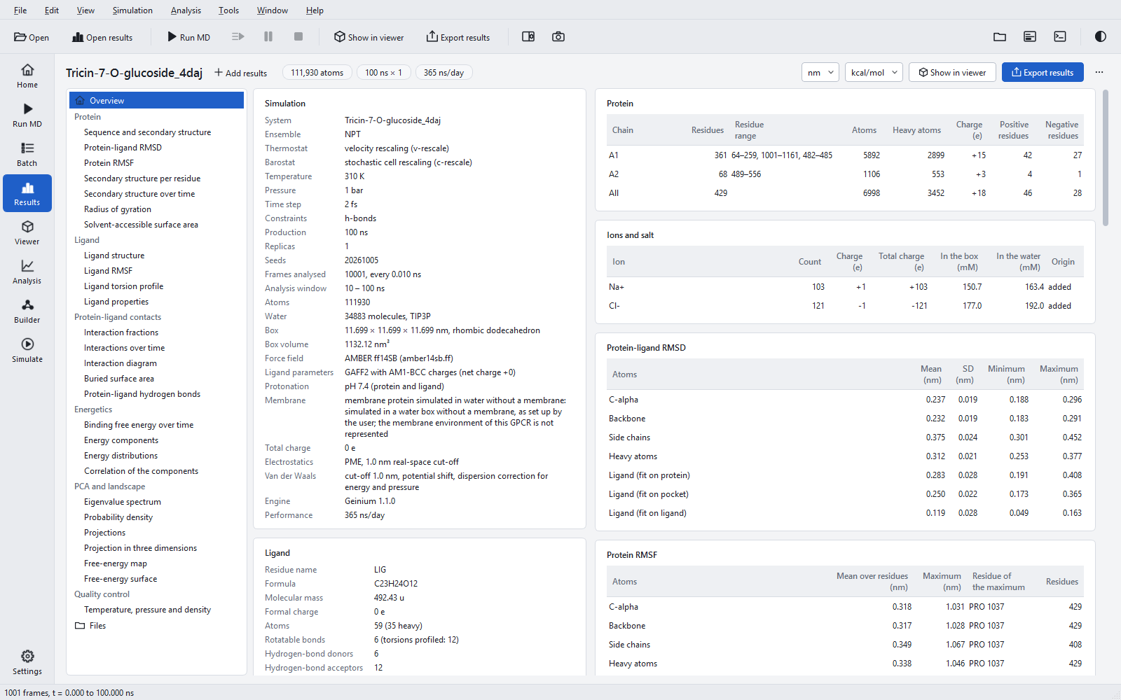
The overview is the first entry of the navigation. It shows, as compact cards, the tables that open the PDF report: Simulation (system, ensemble, thermostat and barostat, temperature, pressure, time step, constraints, production length, replicas and seeds, frames analysed, analysis window, atoms, water model, box, force field, ligand parameters, protonation, membrane, total charge, electrostatics, van der Waals treatment, engine and performance), Protein (one row per molecule with its residue ranges, atoms and charge), Ligand, Ions and salt and, for a membrane system, Molecules. Below them come the statistics tables of every section. With several jobs open the overview adds the Compounds table, the comparison table and the table of the residues with the highest contact fraction.
Read the Simulation card before any figure. It tells you whether the statistics window, the replica count and the length are what you intended, and whether anything unusual was declared (a membrane protein in water, modelled residues, a removed fusion insert). When the job is exported, the run settings on it (engine, precision, time step, ensemble, temperature, pressure, cut-offs) are checked against the production run input and log.
Reading a figure
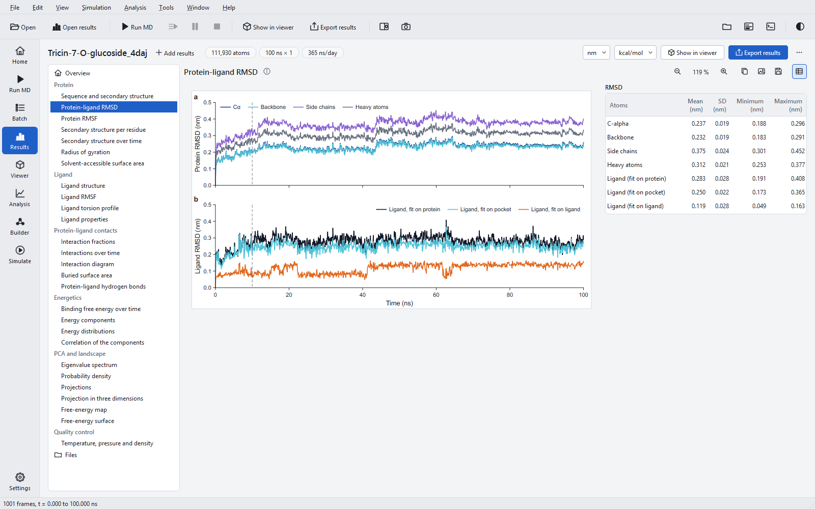
The navigation groups the figures by subject: Comparison (only with several jobs), Protein, Ligand, Protein-ligand contacts, Energetics, PCA and landscape and Quality control, then Files. A figure that can never apply to the job (a ligand figure of a protein-only job, a comparison figure of a single job) is not listed. A figure whose data are missing is listed but greyed, and its tooltip says why.
The figure is drawn on a white sheet in both themes, at the aspect ratio it has in print, and never larger than 1.75 times its printed size when fitted. Ctrl and the mouse wheel zoom between 25 % and 400 %, and a double-click fits the figure to the view again.
| Control | What it does |
|---|---|
| Information icon beside the title | Shows the caption of the figure and its notes as a tooltip: exactly what is plotted, and anything that was left out. |
| Replica | Appears when the job has several replicas: all replicas (one line per replica) or a single one. |
| Part arrows and "1 / 2" | Appears for figures that come in parts, such as the torsion profile of a ligand with more than six torsions. |
| Threshold | Appears on the interaction diagram only: the smallest occupancy, in per cent, for an interaction to be drawn. |
| Zoom out, zoom percentage, Zoom in | Zoom by steps; clicking the percentage fits the figure. |
| Copy image | Puts the figure on the clipboard at 300 dpi (also Ctrl+Shift+C). |
| Save image | Writes the figure as PNG at 300 or 600 dpi, SVG or PDF (also Ctrl+Shift+E). The files are the ones the export writes. |
| Save data | Writes the numbers behind the figure as CSV, in the units chosen in the header. |
| Statistics | Shows or hides the statistics table beside the figure. |

The statistics tables
Each section of figures has one statistics table. With one replica a row gives the mean and the standard deviation over the frames of the window (the population standard deviation). With several replicas it gives the mean of the replica means and the sample standard deviation between the replicas. The note under the table says which, and names the window.
analysis.start_ns in the project (see Project file keys).A standard deviation over the frames of one trajectory describes how much a quantity fluctuates, not how well its mean is known: consecutive frames are strongly correlated, so one run of 100 ns gives far fewer independent samples than it has frames. For an uncertainty of a mean, run independent replicas and use the spread between them.
Units
The two drop-down lists in the header choose one length unit (nm or Å) and one energy unit (kcal/mol or kJ/mol). The choice applies at once to every figure axis, every table and every CSV written with Save data, and it is the default of the export dialog. Time is always in ns. Degrees, kelvin, bar, kg/m³, per cent, elementary charges, atomic mass units, mM and kT keep their units. The defaults are nm and kcal/mol. The files inside the job folder are not touched: they stay in nm, ps and kJ/mol whatever is shown.
Missing analyses
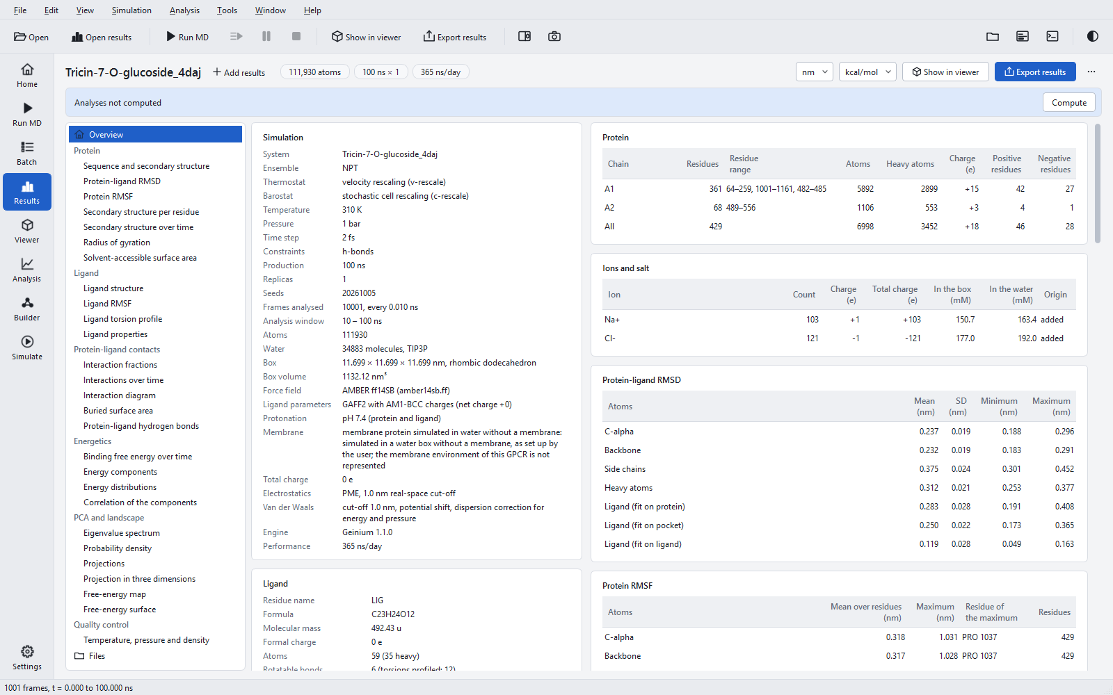
The figures are made from detail analyses that the pipeline computes after the simulation. When they are missing the band offers Compute; when they were made by an older version it says Analyses were made by an older version and must be recomputed and offers Recompute. Either runs the interaction analysis and the detail analyses with a Cancel button; the simulation itself is never repeated. For the 100 ns example with 1001 trajectory frames this took about ten seconds. When the analyses cannot be made from the files that are present, the band says Analyses not available.
Recompute old analyses before comparing a job with a newer one. Definitions change between versions (since 1.1.0 the first 10 % of the run is left out of the statistics and a fusion insert is left out of the fits), and two jobs analysed by different versions are not comparable number for number.
Several results side by side
Add results opens another job beside the open one; Add results folder in the … menu adds a folder of jobs. The job name in the header becomes a drop-down list (the compound selector) that switches every figure and table to another job, and the navigation gains the Comparison group with the figures that put all compounds on common axes. The status bar says how many results are open. Everything about comparisons, and what makes one fair, is on the page Comparing compounds.
Files
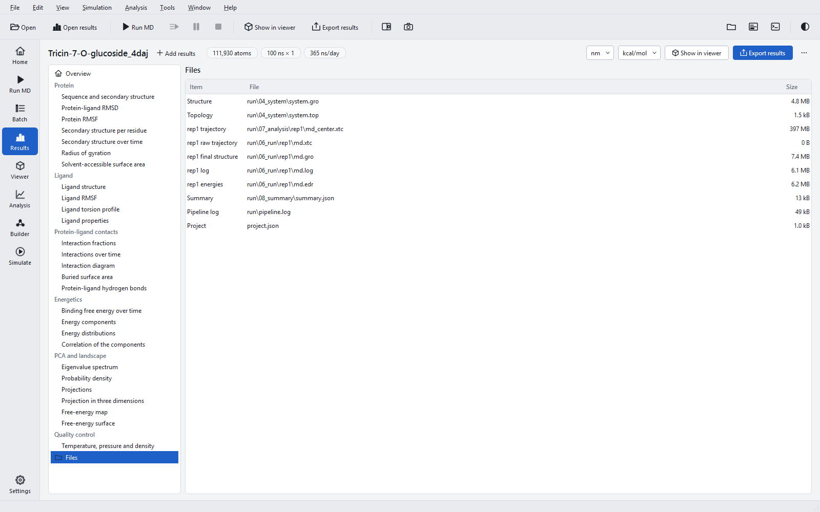
The last entry of the navigation lists the files of the job in a table with the columns Item, File and Size. A double-click opens a file. Once the job has been exported, the report and the results package are listed first.
Show in viewer
Show in viewer (also Analysis > Show in 3D viewer, Ctrl+Shift+V) loads the system structure, the topology and the trajectory of the first replica into the 3-D viewer, and the status bar confirms it, for example "Tricin-7-O-glucoside_4daj: structure and trajectory of rep1 loaded". The centred trajectory written by the analysis stage is shown as it is; when only the raw trajectory exists, the viewer makes molecules whole and centres the solute itself. F4 puts the viewer beside the Results page, so a figure and the structure can be looked at together; see The 3-D viewer and playback.
Result bundles (.gnm)
A result bundle is one file that reopens a job on any PC. File > Save result bundle (.gnm) (Ctrl+Shift+B) writes it from the open job. The dialog asks for the file and for the trajectory: Thinned to a number of frames per replica (500 by default, taken at an even stride) or Every frame. Under Advanced, Run inputs (.mdtpr) and Energy files (.edr) can be added. A bundle holds the job folder without checkpoints and raw trajectories, one centred trajectory per replica, the detail tables and the results package, and records a SHA-256 checksum for every entry.
Opening a bundle unpacks it once into %LOCALAPPDATA%\Geinium\Geinium\cache\bundles and checks every checksum. Tools > Check a result bundle (.gnm) verifies a file without opening it, and Tools > Clear the bundle cache removes the unpacked copies.