Trajectory analyses
What each analysis of the protein measures, on which atoms, after which fit, and over which part of the run its statistics are taken.
This page describes the analyses of the protein and of the run as a whole: deviation and fluctuation, secondary structure, compactness and surfaces, protein-ligand hydrogen bonds, and the temperature, pressure and density of the run. For each figure it says what is plotted and exactly how it is defined, how to read it, what typical values look like, and where it misleads. The figures are those of the example job Tricin-7-O-glucoside_4daj, a 100 ns run of the M3 muscarinic receptor (PDB 4DAJ) with its T4 lysozyme fusion insert, in a water box at 310 K.
Reference structure, fits and the statistics window
Every deviation is measured from the reference structure: the coordinates at the start of the production run, with every molecule made whole. Before a deviation or a fluctuation is computed, each frame is superimposed on the reference by a mass-weighted least-squares fit on the fit group, by default the protein backbone (atoms N, Cα and C of the receptor).
A fusion insert, a soluble protein engineered into a loop to help crystallisation, is taken out of the fit group, out of the four atom sets of the protein RMSD, out of the Cα fit of the RMSF and out of the PCA. In 4DAJ this is the T4 lysozyme domain, residues 1001 to 1161. The insert hangs on two flexible links and moves as a body relative to the receptor; fitted together with the receptor it would tilt the superposition and inflate every number. In the example job, removing it from the fits lowered the mean ligand RMSD after the protein fit from 0.41 to 0.28 nm. The RMSF is still reported for every residue of the insert. How the program recognises an insert is described under Structure preparation.
With one replica the tables give the mean and the population standard deviation over the frames of the window. With several replicas they give the mean of the replica means and the sample standard deviation between the replicas; that second number is the one to quote as an uncertainty. When the job has fewer than three replicas, or when the RMSD drifts between the two halves of the window by more than twice its block-averaged standard error, the export log says so (rules replicas.min3 and convergence.drift; see Exporting results).
Sequence and secondary structure
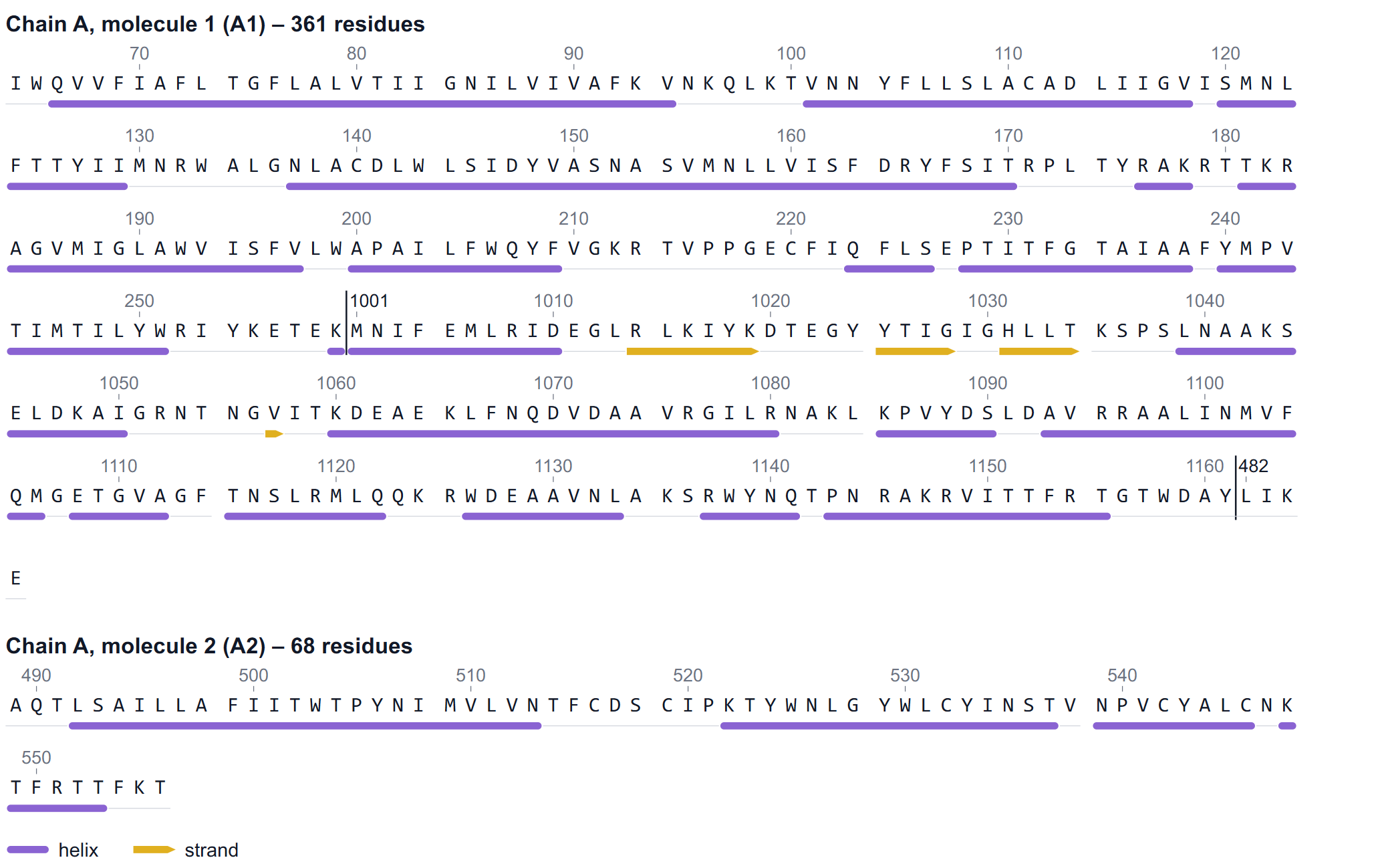
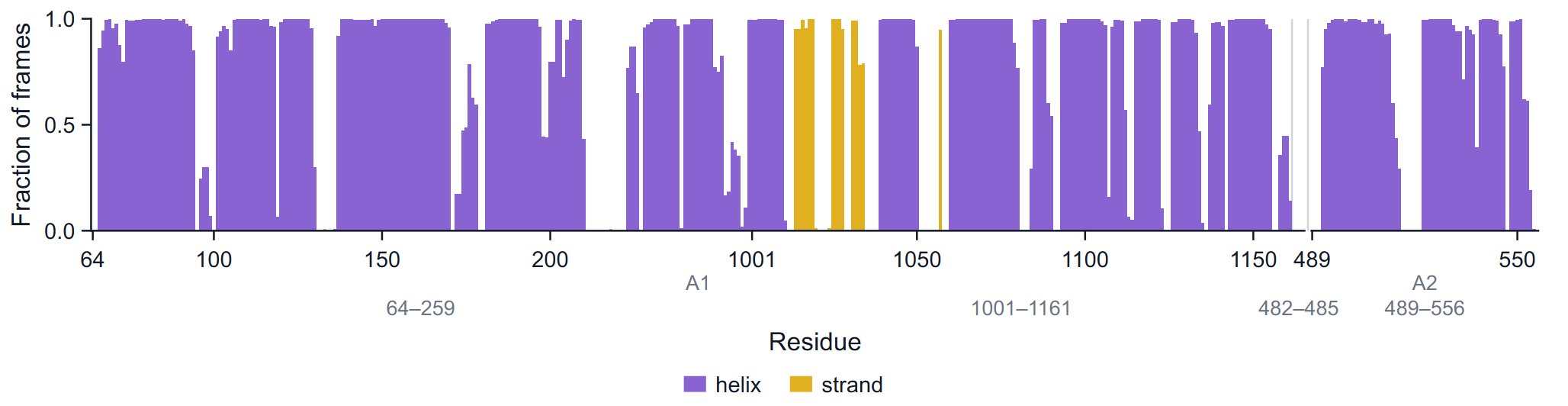
The first figure of the Protein group is not a time series but a map of the protein: its one-letter sequence in rows of 60 residues, the residue number above every tenth residue, and a track underneath with a violet bar for every helix and a gold arrow, pointing to the C-terminus, for every strand. A residue is drawn as helix or strand when it is in that class in at least half of the analysed frames. Where the numbering jumps inside a molecule, a divider and the first number after the jump are drawn; a new molecule (in the pipeline every chain break becomes its own capped molecule) gets its own heading such as "Chain A, molecule 2 (A2)".
Use it to orient yourself before reading the residue axes of the other figures, and to check that the simulated construct is the one you meant: modelled or missing residues, a kept or removed fusion insert, and the chain breaks are all visible here.
RMSD
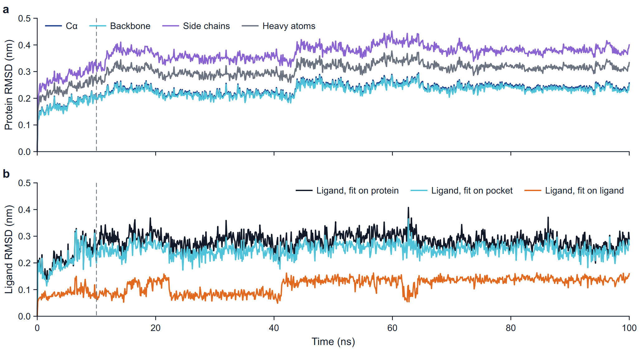
The root-mean-square deviation of a set of N atoms after the fit is RMSD(t) = sqrt( Σ mi |ri(t) − riref|² / Σ mi ), mass-weighted, against the reference structure.
| Series | Atoms | Fit | What it tells you |
|---|---|---|---|
| Cα | Cα atoms of the receptor | Backbone | Overall drift of the fold. |
| Backbone | N, Cα, C of the receptor | Backbone | The same, the usual number to quote for the protein. |
| Side chains | Side-chain heavy atoms | Backbone | Rearrangement of side chains; always larger than the backbone value. |
| Heavy atoms | All heavy atoms of the receptor | Backbone | Backbone and side chains together. |
| Ligand, fit on protein | Ligand heavy atoms | Protein backbone | How far the ligand moved in the frame of the whole protein: displacement in the pocket plus any motion of the pocket relative to the rest of the protein. |
| Ligand, fit on pocket | Ligand heavy atoms | Cα atoms of the pocket | How far the ligand moved relative to the residues that surround it. The pocket is every residue with an atom within 0.6 nm of a ligand heavy atom in the reference. |
| Ligand, fit on ligand | Ligand heavy atoms | The ligand heavy atoms | Change of the shape of the ligand alone, with its position and orientation removed. |
The fusion insert is excluded from the four protein sets and from the protein fit. For the RMSD after the protein fit the ligand is taken in the periodic image nearest to its reference position, so a ligand that crosses the box boundary does not produce a jump of a box length.
How to read it
- Protein curves. A rise over the first nanoseconds followed by a plateau is normal: the structure relaxes from the crystal environment into solution and then fluctuates about a new average. For a well-folded globular domain the backbone RMSD usually levels off somewhere between 0.1 and 0.3 nm. A curve that is still climbing at the end, or steps to a new level, points to a conformational change, a flexible part in the atom set, or two domains moving relative to each other. In the example the backbone settles at 0.232 ± 0.019 nm (10 to 100 ns) with a small step at about 43 ns.
- Ligand curves. Read the three together. A ligand that keeps its pose stays low and flat after the protein fit; values that climb past roughly 0.3 to 0.5 nm and keep rising mean the ligand is shifting or leaving the site. When the protein-fit curve is high but the pocket-fit curve is low, the pocket moved and took the ligand with it. When the ligand-fit curve changes level, the ligand changed its own conformation; look for the torsion that switched at the same time on the page Ligand analyses. In the example the means are 0.283 (protein fit), 0.250 (pocket fit) and 0.119 nm (ligand fit).
- The table gives the mean, the standard deviation, the minimum and the maximum of every series over the window, with the number of atoms in each set.
Pitfalls: when the fit group spans several molecules (4DAJ has two, A1 and A2, after the chain break at 486 to 488), a motion of one molecule relative to the other enters the RMSD of both; the export log names this case (rule fit.molecules). Long flexible termini or unstructured loops in the atom set raise the RMSD without any change of the fold. The first frame is the reference, so the curves start at zero by construction.
RMSF
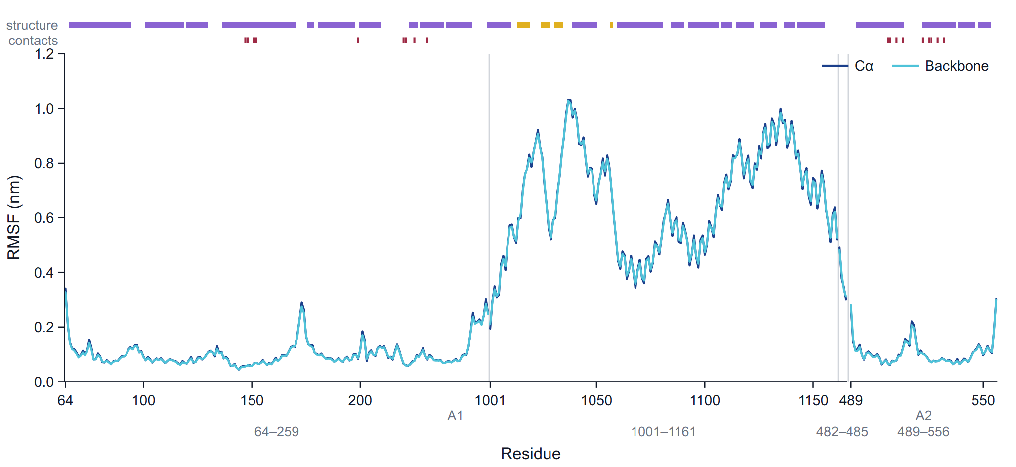
The root-mean-square fluctuation of an atom is RMSF = sqrt( < |r(t) − <r>|² > ), the deviation from its mean position over the frames of the window, after each frame has been fitted. The Cα series uses the Cα atoms, fitted on the Cα atoms; the backbone series uses the backbone atoms of each residue after the backbone fit, combined into one value per residue as the square root of the mass-weighted mean square fluctuation. The table adds the side chains and all heavy atoms of each residue. The fusion insert is out of the fit but keeps its RMSF.
The x axis is a compact residue axis: one slot per residue in sequence order, labelled with the residue numbers. A faint line marks every place where the numbering jumps, a wider gap marks a change of molecule, and the molecule names (A1, A2) and the segment ranges are printed under the axis. Two tracks run above the frame: structure (helix and strand residues, by the majority rule) and contacts (a tick at every residue that interacts with the ligand in at least 5 % of the frames).
How to read it
Peaks at the chain termini and at loops are expected; secondary-structure elements and the buried core fluctuate least. Typical Cα values for a folded protein at room or body temperature are 0.05 to 0.15 nm in helices and strands and 0.2 to 0.4 nm or more in exposed loops and termini. Compare the contact track with the curve: binding-site residues that fluctuate strongly suggest a loosely held ligand or a mobile lid over the pocket. Comparing the RMSF of an apo and a holo run, or of two ligands on the same receptor, shows which regions a ligand stiffens.
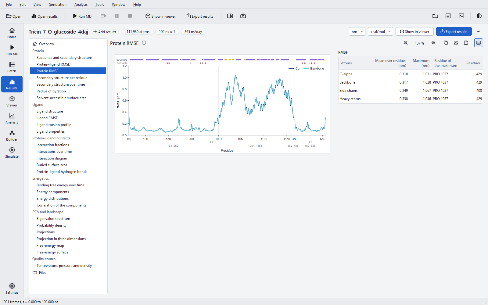
Pitfalls: the RMSF is computed over the window only, so an event in the first 10 % is not in it. A domain that moves as a body, such as the excluded insert, gets large values everywhere; that measures its motion relative to the fitted part, not its internal flexibility. The mean over residues in the table (0.318 nm for Cα in the example) is dominated by such a domain; quote the receptor part separately if it matters.
Secondary structure
Secondary structure is assigned in every frame with the DSSP method (Kabsch and Sander, 1983), which finds backbone hydrogen bonds from their electrostatic energy and classifies each residue as α-helix (H), 310-helix (G), π-helix (I), strand (E), bridge (B), turn (T), bend (S), polyproline helix (P) or loop. The figures use two classes: helix = H + G + I and strand = E + B. The assignment of the program was compared with an established reference program: no letter differed on any of the validation trajectories.
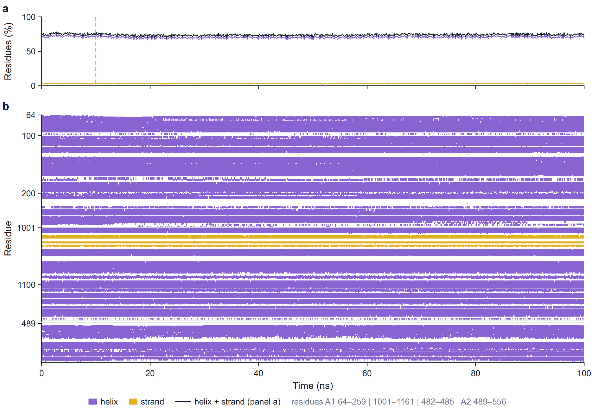
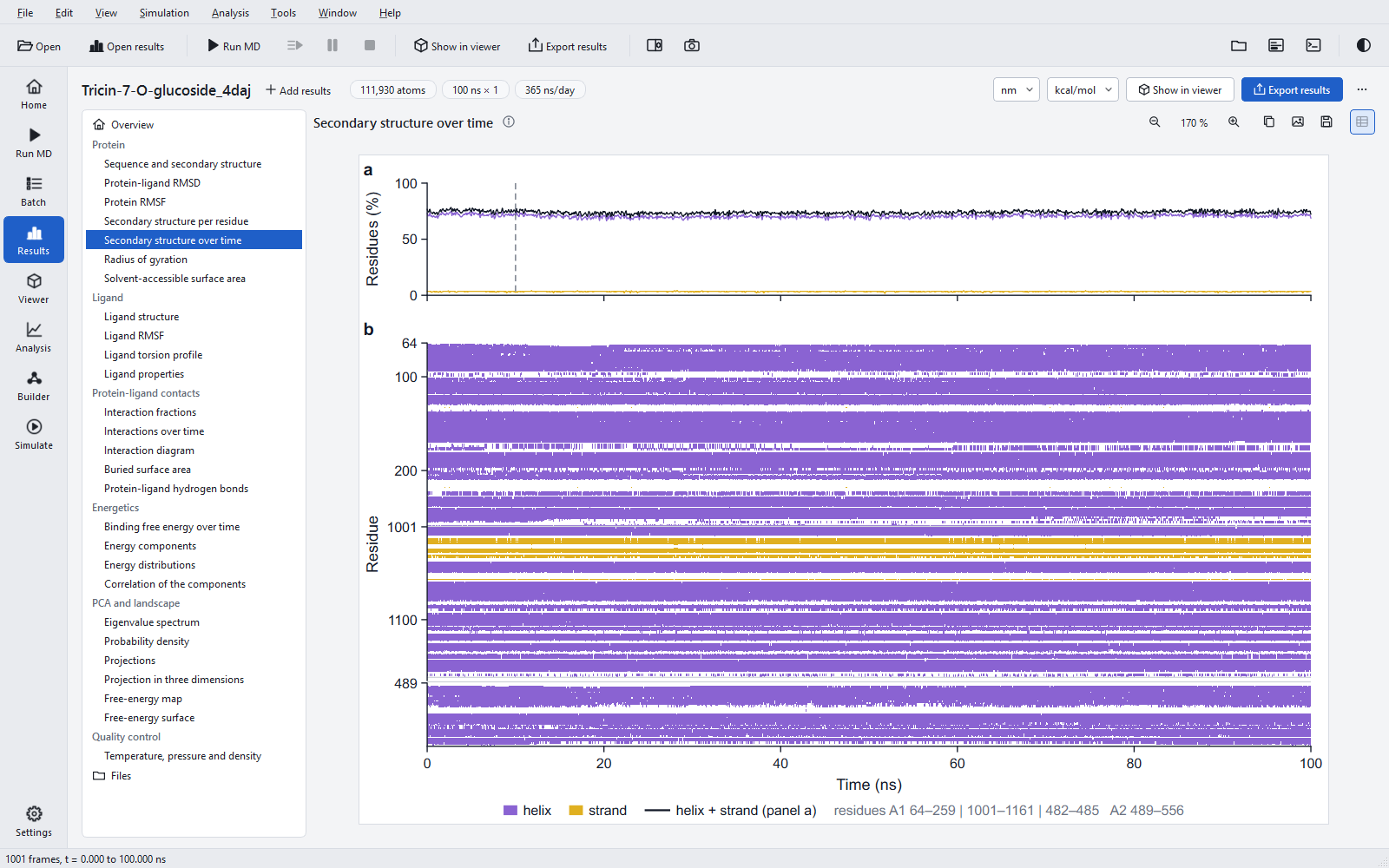
In the timeline map, a run with more than 600 frames is binned along time and each cell takes the class of most of its frames; the caption note then says so. The table of the section gives the mean, standard deviation, minimum and maximum of helix, strand and helix + strand content in per cent over the window.
How to read it: a stable protein shows flat lines in panel a and unbroken bands in panel b. A band that thins out or breaks up over time is a helix unwinding or a sheet coming apart; look at whether it lies near the ligand (contact track of the RMSF) before calling it significant. Flickering between H and T at helix ends is normal and is why the per-residue fractions near the ends are below 1.
Radius of gyration
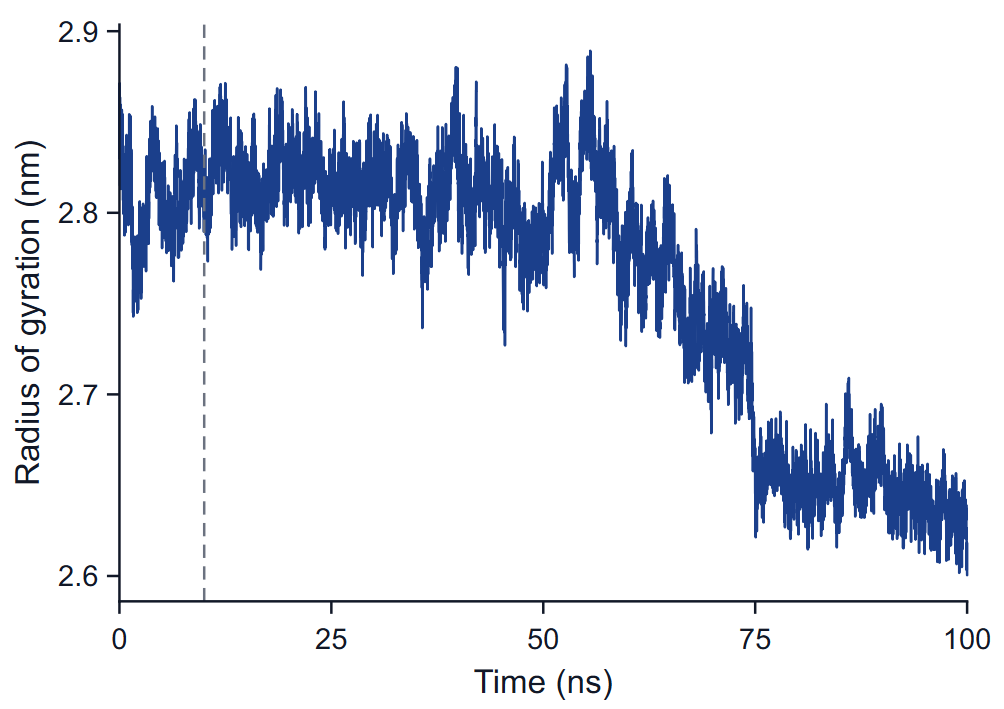
The radius of gyration is the mass-weighted root-mean-square distance of the atoms of the receptor from their centre of mass, Rg = sqrt( Σ mi |ri − rcom|² / Σ mi ), per frame. It needs no fit. Its x, y and z components are kept in the raw data.
How to read it: a folded protein keeps a nearly constant Rg with fluctuations of a few hundredths of a nanometre. A steady rise means unfolding or domains moving apart; a drop means compaction or domains closing. In a fusion construct the relative position of the two domains dominates Rg, so a step like the one at 60 to 75 ns in the example is first a question about the insert; play the trajectory around that time in the viewer before drawing a conclusion about the receptor.
Surfaces
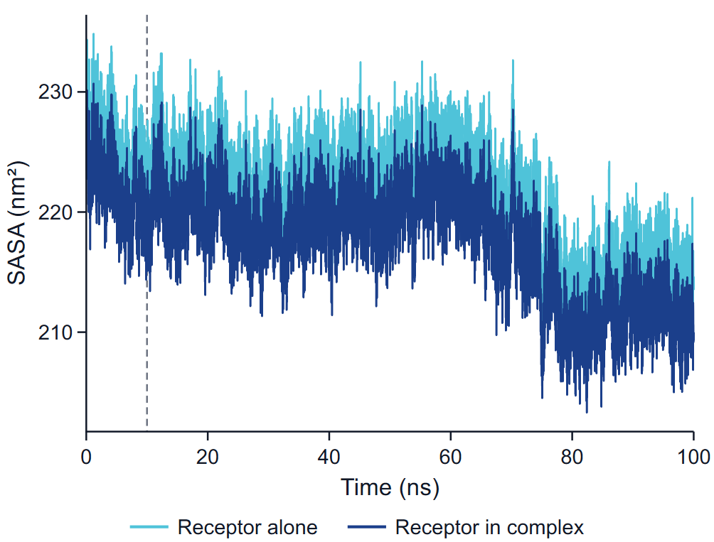
The solvent-accessible surface area is the area traced by the centre of a probe sphere of radius 0.14 nm rolled over the van der Waals spheres of the atoms, computed by dot counting with 32 points per atom. Water and ions are not part of the surface. Two series are drawn:
- Receptor alone: the surface of the receptor computed without the ligand, in the coordinates of the frame.
- Receptor in complex: the part of the surface of receptor + ligand that belongs to receptor atoms.
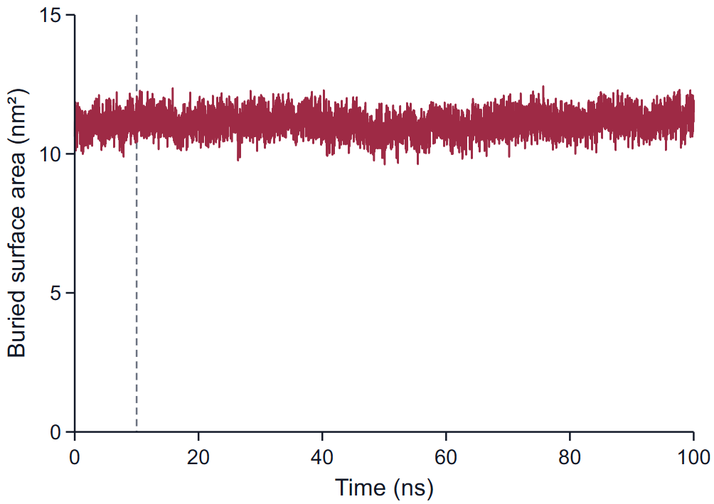
The buried surface area is SASA(receptor alone) + SASA(ligand alone) − SASA(complex), all from the same coordinates. It counts the area lost on both sides of the interface, so it is about twice the area of the contact patch. Typical values for a drug-sized ligand fully in a pocket are several square nanometres; 11 nm² in the example reflects a large glycosylated ligand. A falling buried area is the surface sign of a ligand that is working its way out.
The table Protein compactness and surface gives the mean and standard deviation of Rg, both receptor surfaces, the buried area and the hydrogen-bond count over the window. Note that the ligand surfaces on the Ligand properties page are computed with a finer dot density than these whole-system surfaces, and the two sets are not compared number for number.
Protein-ligand hydrogen bonds
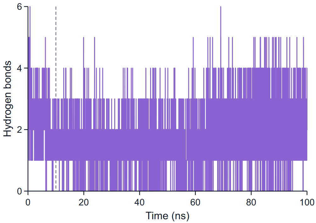
A hydrogen bond is counted between a donor D (N or O carrying a hydrogen H) and an acceptor A (N or O), one of them in the receptor and the other in the ligand, when the distance D···A is at most 0.35 nm and the angle H-D···A at most 30°. The figure plots the number of such bonds in every frame as a step line.
How to read it: the mean over the window (1.68 ± 0.92 in the example) says how many hydrogen bonds the ligand typically holds; a count that falls to zero and stays there means the polar anchoring was lost. Which bonds they are, and how often each one is present, is on the page Protein-ligand interactions. A count is not an occupancy: three short-lived bonds and one permanent bond can give the same mean.
Run quality
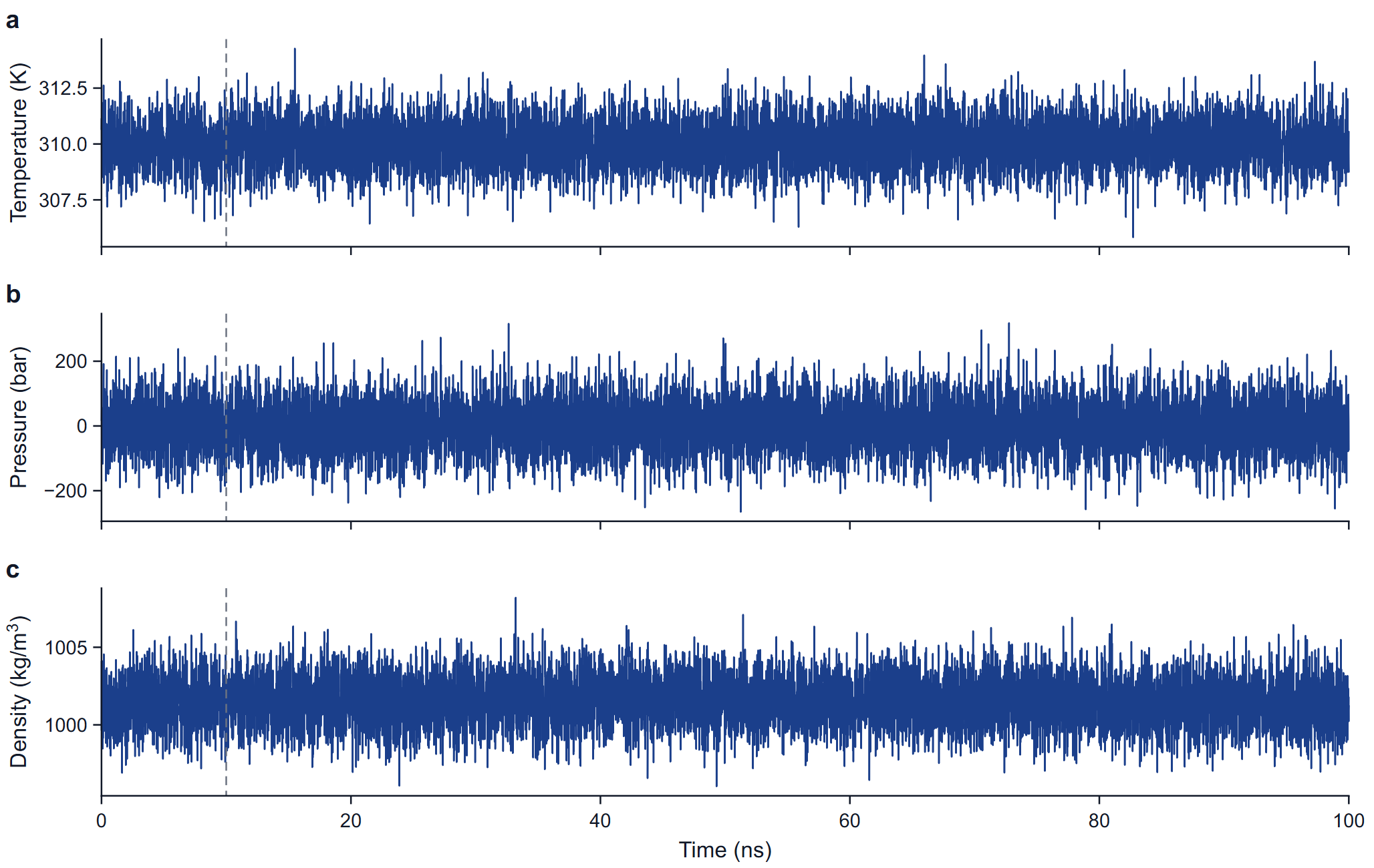
The three panels plot the temperature (K), the pressure (bar) and the density (kg/m³) at every point written to the energy file of the production run. No value is smoothed and none is removed: an isolated extreme first value is drawn, named in the caption and kept in the statistics, and the table note gives the standard deviation of the other frames as well.
What normal looks like: the mean temperature within a fraction of a kelvin of the target; a mean pressure within a few bar of the reference with instantaneous values spread over tens to hundreds of bar (the spread shrinks with system size and is not a fault); a density that is flat after equilibration, near 1000 to 1020 kg/m³ for a protein in TIP3P water. A drift in density or a temperature offset is a reason to look at the equilibration before reading any other figure. The live plots during a run are described under Monitoring a running job.