PCA and free-energy landscape
Principal components of the protein motion and the free-energy landscape on the first two of them.
Principal component analysis (PCA) reduces the motion of a protein to a few collective directions that carry most of its variance. The projection of each frame on the first components shows which conformations the run visited and in which order, and a histogram over the first two gives a free-energy landscape. Both describe the frames that were sampled; with a single run of 100 ns they are rarely converged, and this page shows how to tell.
What is analysed
The atoms are the Cα atoms of the receptor, without a fusion insert (at most 3000 atoms). Every frame of the window is fitted on the same atoms, without mass weighting, to the reference structure of the first replica. The covariance matrix of the positions over the frames of all replicas is diagonalised; its eigenvectors are the principal components (PC1, PC2 …) and its eigenvalues, in nm², the variance along each; frames are fitted in the same way before they are projected. The sign of each eigenvector is fixed so that its component of largest magnitude is positive. The projection of a frame on a component is pk(t) = ek · (x(t) − <x>), in nm.
Density and landscape use the frames of the window; the projections are written and drawn for every frame of the run, so the scatter plots show the first 10 % as well.
Eigenvalue spectrum
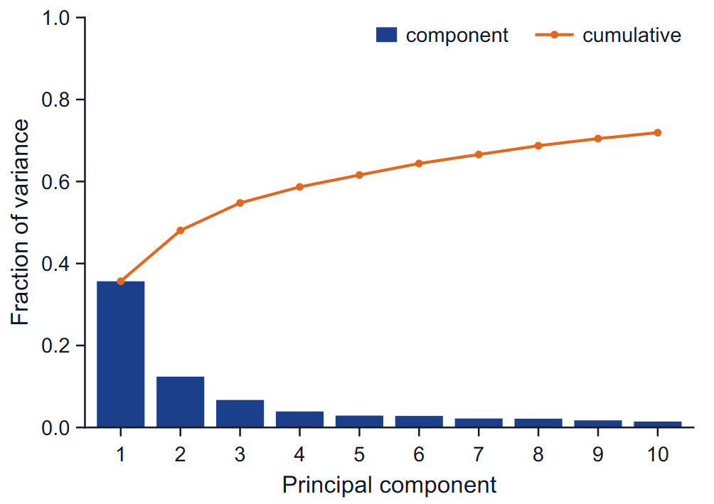
The bars are the fraction of the total variance carried by each of the first ten components, the line the cumulative fraction. A steep drop after the first one or two components means the motion is dominated by a few collective modes and a two-dimensional projection is a fair summary; a flat spectrum means it is not. The table gives the eigenvalue, the percentage and the cumulative percentage of PC1 to PC5, and the cosine content of each.
Probability density
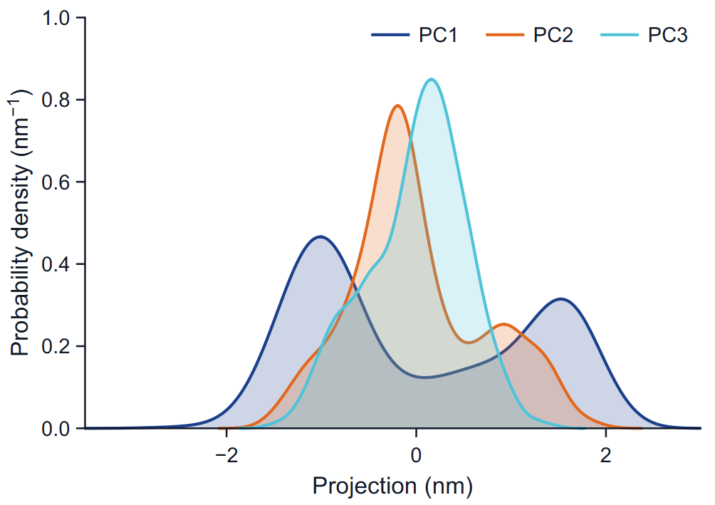
Each curve is a kernel density estimate of the projections on one component: Gaussian kernels with Silverman's bandwidth, h = 0.9 min(SD, IQR / 1.34) n−1/5, on 256 points, in inverse nm. One peak means one region of conformations along that direction; several peaks, several regions. Unequal peak heights reflect how long the run stayed in each, not necessarily how stable each is.
Projections
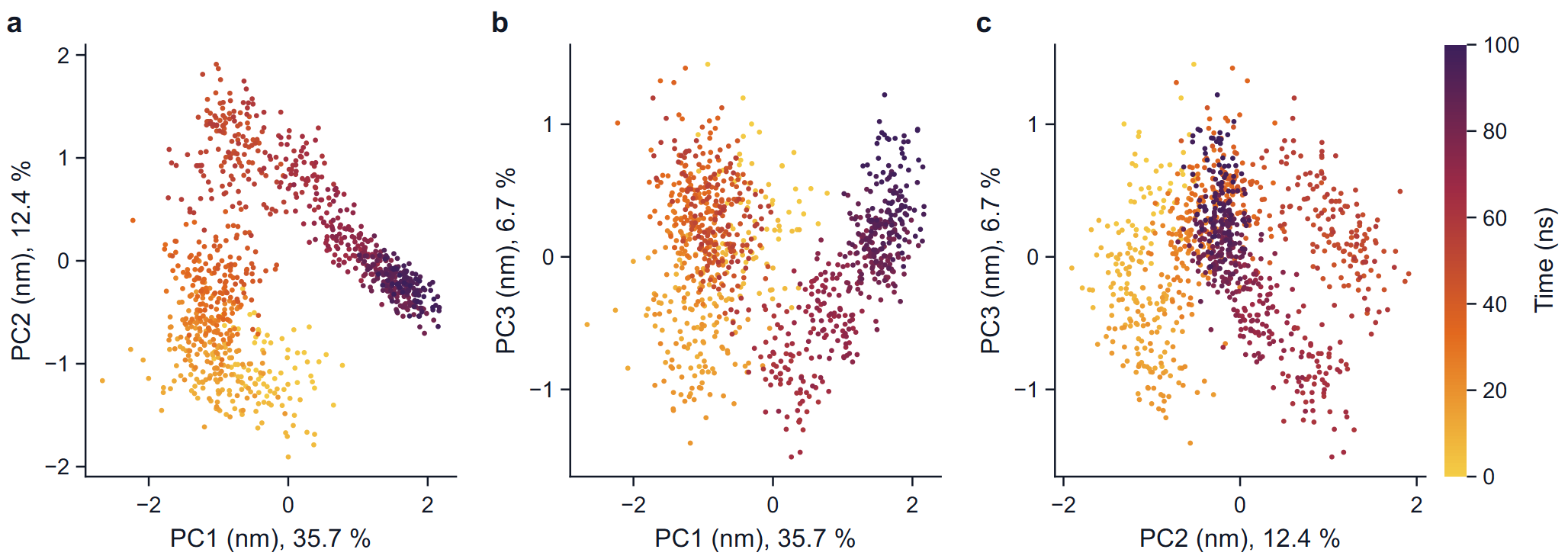
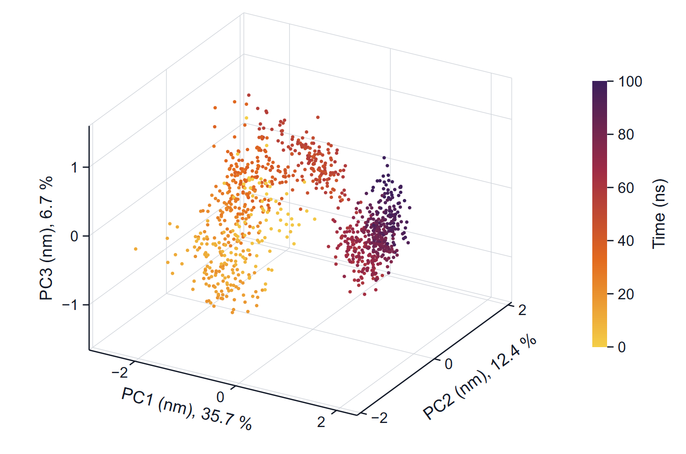
Each point is a frame. With one replica the colour is the time of the frame; with several replicas the colour is the replica, so that you can see whether independent runs explore the same regions. The axis labels carry the fraction of the variance of each component.
How to read it: a converged sampling looks like a cloud in which early and late colours are mixed. A path that moves steadily through the plot, with colours in sequence, is a drift or a slow transition. Several replicas that cover the same region are the best evidence that the region is representative.
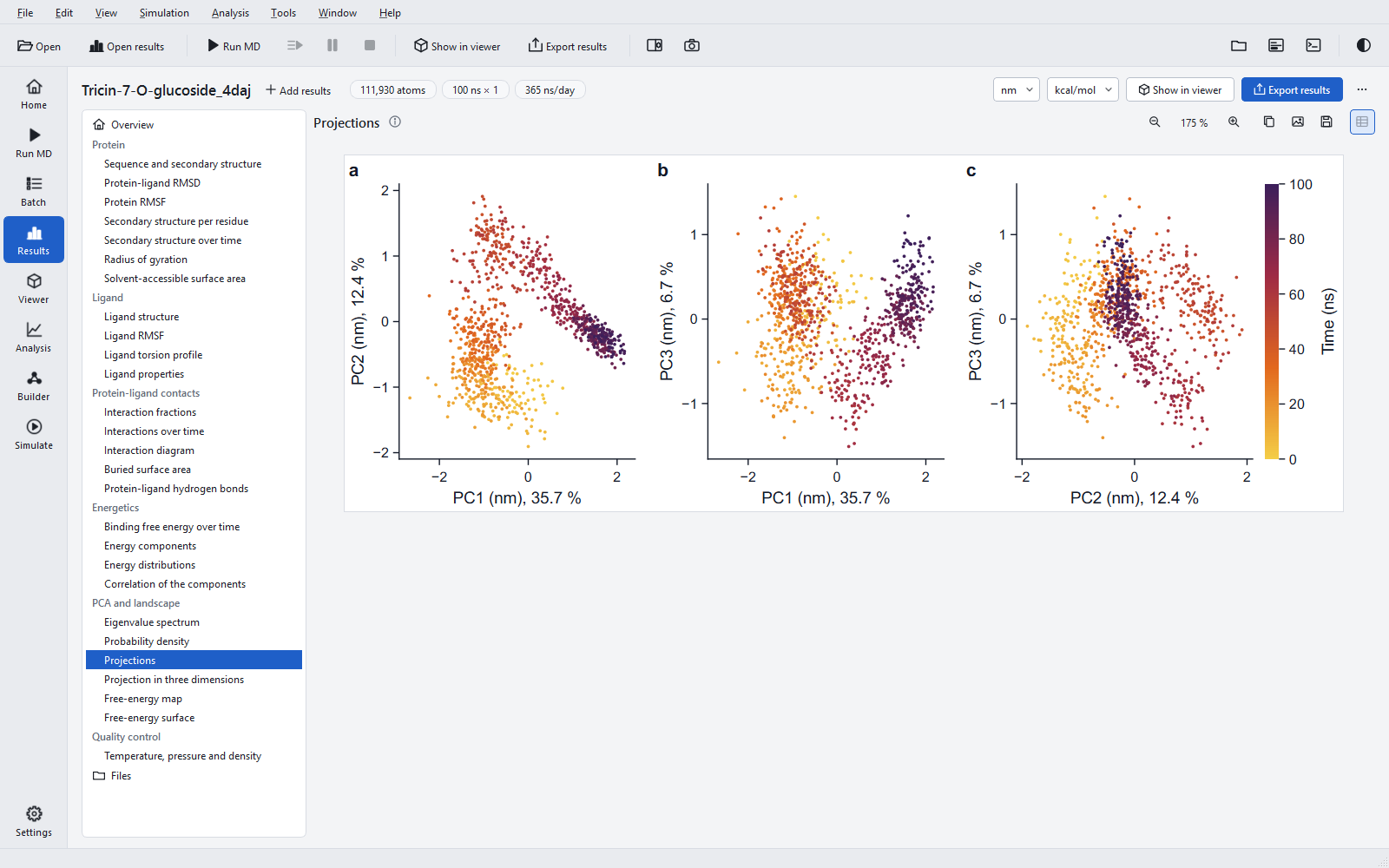
Cosine content and convergence
For each replica the program computes the cosine content of the projections on the first components (Hess, 2000): how closely the projection over time resembles a half cosine. Random diffusion produces exactly such shapes, so a cosine content close to 1 means the principal component describes a slow drift rather than fluctuations about an equilibrium, and the sampling along it is not converged. The 100 ns jobs measured during development had values from 0.63 to 0.86; the example has 0.86 for PC1 and 0.67 for PC2. Values like these are the normal state of a single 100 ns run of a large protein, and they are the reason the landscape below describes the sampled frames and not an equilibrium distribution.
Free-energy landscape
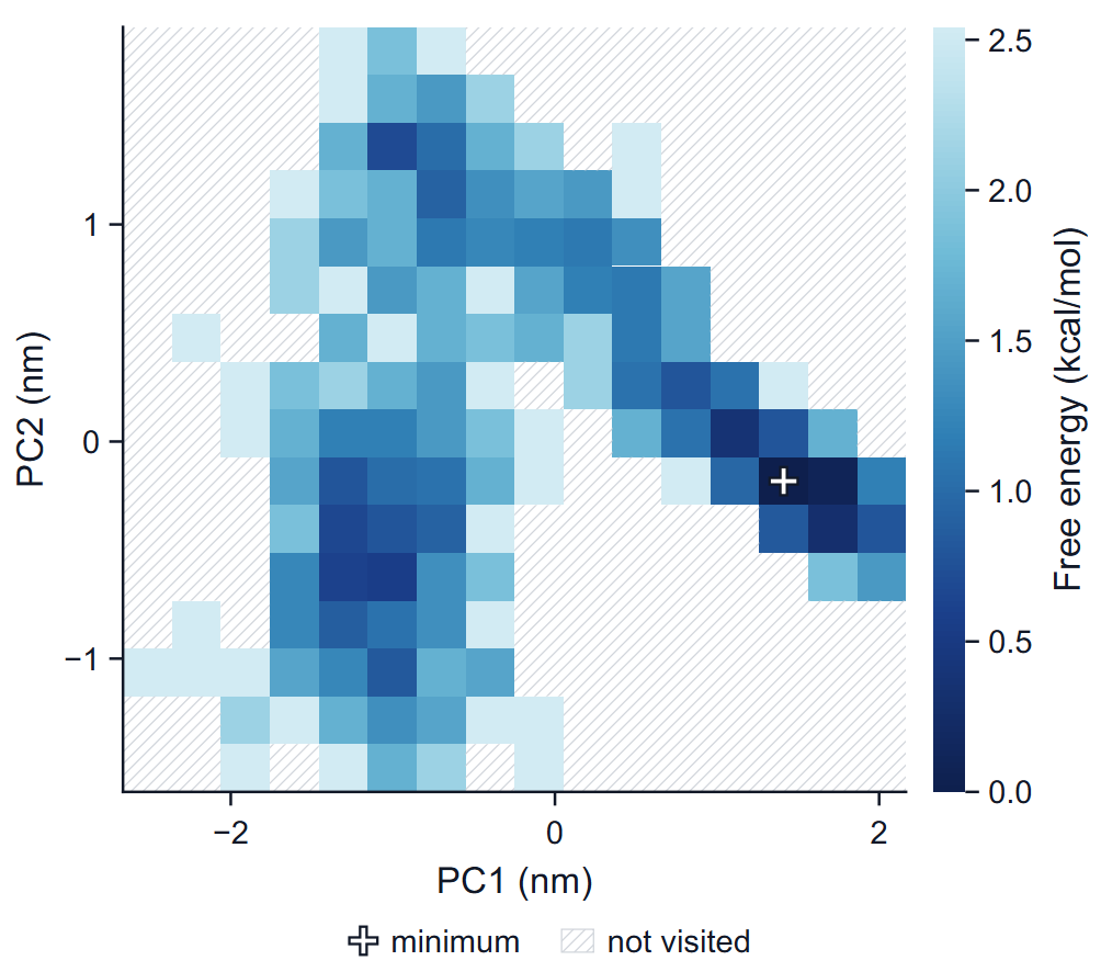
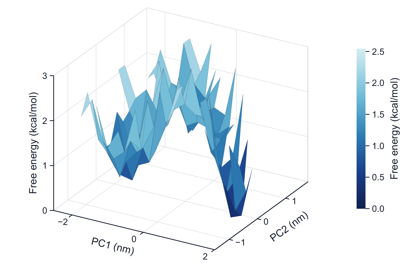
The frames of the window are counted in a two-dimensional histogram over PC1 and PC2, and each bin gets G = −kT ln(P / Pmax), where P is the fraction of frames in the bin, Pmax that of the most populated bin and T the temperature of the production run. The minimum is therefore 0 by definition. The number of bins per axis is floor(sqrt(frames / 5)), but at least 16 and at most 64; the range is the range of the projections. A bin without frames has no free energy: it is hatched in the map and left out of the surface, never painted with the highest colour.
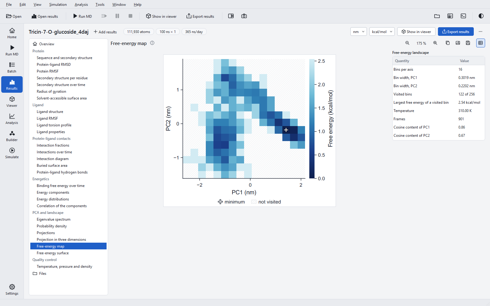
How to read it
Dark basins are regions where the run spent much of its time; the colour difference between two basins is the free-energy difference that their populations imply, in the energy unit of the export (kT = 0.62 kcal/mol = 2.58 kJ/mol at 310 K). Barriers between basins are only estimated if the run crossed them several times.
Limits
- No error bars are drawn: the frames of a trajectory are correlated, and the densities and the landscape describe the analysed frames only.
- The components are those of this run; two jobs have different components, so their landscapes are not drawn on common axes.
- For a statement about conformational populations, run several replicas, check that their projections overlap, and look at the cosine content of each.
The PCA was validated against an established reference program (eigenvalues to a relative 4.3 × 10⁻⁶, projections to 1.1 × 10⁻⁵ nm, the print precision of that program), and the density and the histogram were recomputed independently.