The design workspace
The workspace is where a built design lives. The tree on the left is the table of contents for one experiment; the panel on the right shows whichever page you select. This reference covers the run sheet and the Information branch. Analysis and optimization each have their own pages.
When a design is built, or when you open a saved .ogdx file, you land on
Design (Actual), the top node of the tree. That node holds the run sheet, the single
most important screen in the software. Everything below it reads from the same design, so the moment
you change a value here, the summary, the plots and the analyses see the change too.
The run sheet
Each row of the run sheet is one experiment. The software has already worked out the factor settings for every run; your job is to carry out the runs and type the measured responses into the last columns. The worked example used throughout this documentation is a face centred central composite design on two factors, A: HPMC E15 (2 to 4 % w/v) and B: Glycerol Ester (0.5 to 1.5 % w/v), with 13 runs including 5 centre points, and two responses, Disintegration Time (sec) and Hardness (N).
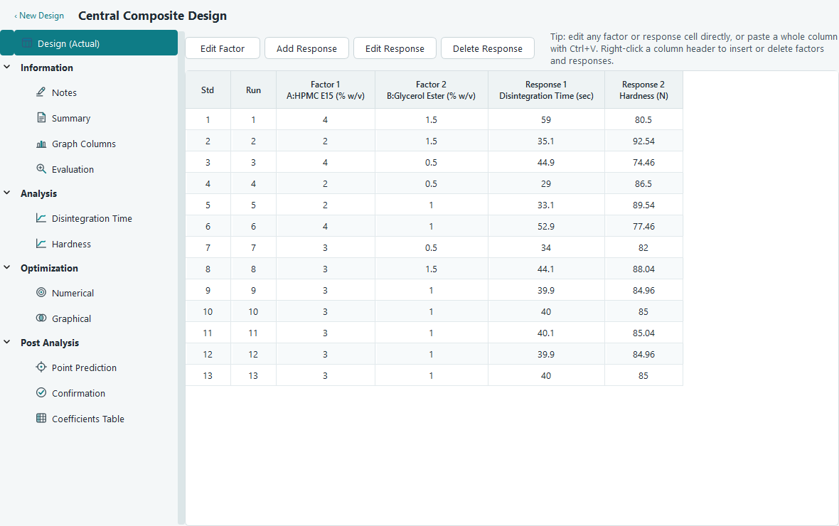
A:HPMC E15 (% w/v) is factor A.Std, Run and the point of randomising
The first two columns are fixed and cannot be edited. Std is the standard order, the tidy textbook order in which the design was generated. Run is the order in which you should actually perform the experiments, and the rows are shown sorted by it.
If your design is split into blocks, a Block column appears between Run and the first factor. It too is read only. The two factor example has no blocks, so you will not see that column there.
Entering and pasting response data
Click a response cell and start typing; you do not need to double click first. Response cells and numeric factor cells accept numbers only, so a stray letter is simply rejected. To bring in a whole column from a spreadsheet, copy it there, click the top response cell here and press Ctrl + V. Paste fills downward and across, following the tab and newline layout of what you copied, and it quietly skips the Std, Run and Block columns so it will not overwrite them.
Cut, copy, paste, undo and redo
The run sheet uses the standard Edit menu and toolbar, so the shortcuts are the ones you already know. Copy and cut work on the block of cells you have selected. Delete clears the selected factor and response cells but leaves Std, Run and Block alone. Undo remembers a long history of cell edits, so you can walk mistakes back one step at a time.
| Action | Shortcut | What it does here |
|---|---|---|
| Copy | Ctrl + C | Copies the selected cells to the clipboard. |
| Cut | Ctrl + X | Copies, then clears the selected cells. |
| Paste | Ctrl + V | Fills cells from the clipboard, skipping Std, Run and Block. |
| Delete | Del | Clears the selected factor and response cells. |
| Undo | Ctrl + Z | Steps back through your cell edits. |
| Redo | Ctrl + Y | Re-applies an edit you undid. |
Right click a cell for the same commands plus Copy with Headings, which puts the column titles on the first line so a paste into a report or a spreadsheet arrives already labelled.
Editing factors and responses
You will not always get the design exactly right the first time. You might rename a factor, add a response you forgot, or drop one you no longer need. A small toolbar sits above the run sheet with Edit Factor, Add Response, Edit Response and Delete Response. For the rest, right click a column, either a cell or its header, and the menu offers Insert and Delete in place.
| Task | How | What changes |
|---|---|---|
| Rename a factor | Select its column, press Edit Factor | Its display name and units only. The range and levels were set when the design was built and stay fixed. |
| Insert a factor | Right click a factor column, Insert Factor, Before or After | Adds a new numeric factor and re-letters the columns A, B, C and so on. |
| Delete a factor | Right click, Delete Factor | Removes the column from every run and re-letters the rest. A design must keep at least one factor. |
| Add a response | Add Response, or right click for Insert Response | Asks for a name and units, then adds an empty column. |
| Edit or delete a response | Select the column, Edit Response or Delete Response | Renames it, or removes the column and its data after a confirmation. |
The tree helps you keep track. Under Analysis each response is tagged (Empty) until it has data, (Analyzed) once you have fitted it, and back to its plain name if an edit has outdated the fit.
The Information branch
The Information section gathers everything that describes the design without analysing it: free notes, a computed summary, quick plots of the raw columns, and a formal evaluation. The first three are covered below; the fourth has its own page, Evaluating a design, because it is worth reading before you commit to the runs.
Notes
Notes is a plain text area for anything the run sheet cannot hold: what you were trying to learn, which batch of raw material you used, a reminder about a run that went wrong. Write in your own words; there is no structure to follow.
Summary
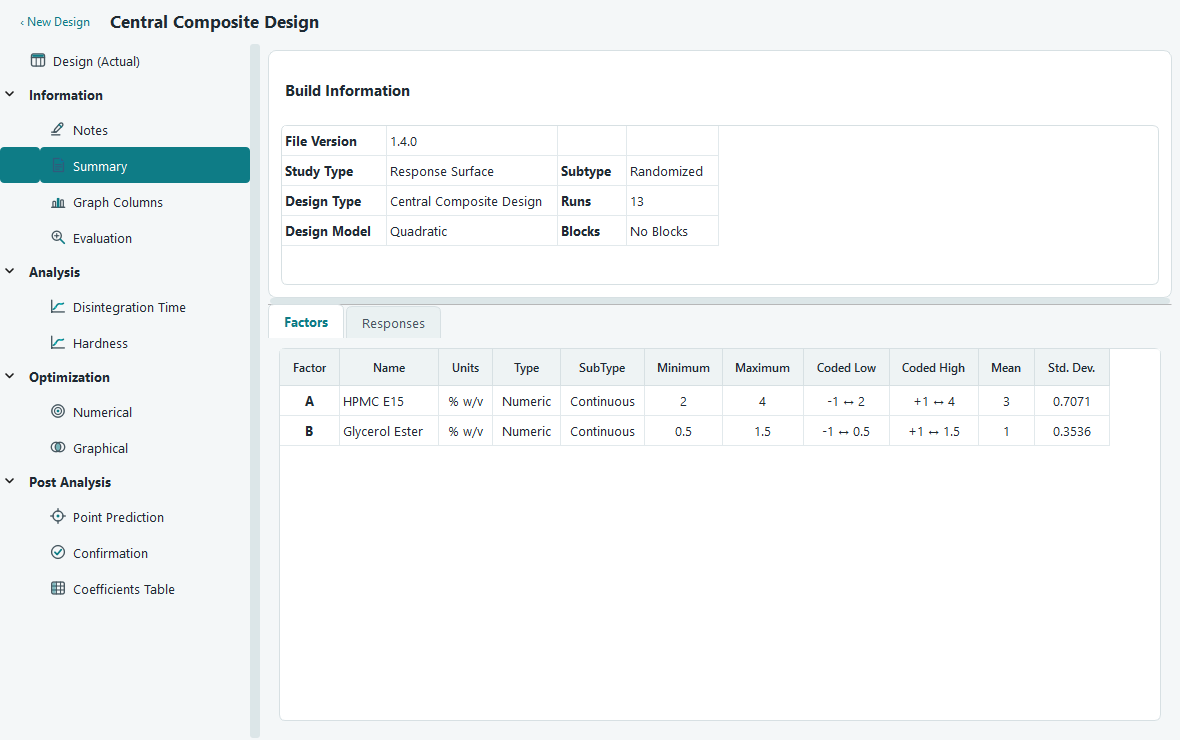
Summary is read only. It reads the design back to you so you can confirm it is what you meant to build. A Build Information panel at the top lists the file version, the study type and its subtype, the design type and run count, the default model, and the block count. Below it, two tabs hold statistics that the software computes straight from the run sheet.
| Tab | Columns |
|---|---|
| Factors | Factor letter, name, units, type and subtype, minimum and maximum, the coded low and high, and the mean and standard deviation of the settings. |
| Responses | Response label, name, units, the count of observations you have entered, the minimum, maximum, mean and standard deviation, and the max to min ratio. |
The response ratio is a quick health check. A large max to min ratio hints that a transform may steady the spread of the data, which is exactly what the Fit Summary tab looks at later in Fit summary, model and ANOVA.
Graph Columns
Graph Columns lets you look at the raw numbers before you fit anything to them. It is the fastest way to catch a typo, a wildly out of range value or a pair of columns that move together. Pick a chart from the tabs across the top, then set the columns from the tool panel on the right. Every column is available: Standard Order, Run, each numeric factor and each response.
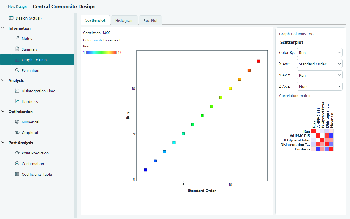
- Scatterplot plots any column against any other and can colour the points by a third. The panel reports the correlation between the two axes so you can put a number on what you see.
- Histogram shows the shape of one column as frequency or as relative percent. Set the number of bins, or press Default to let the software choose from the count of values, and tick the box to print the count above each bar.
- Box Plot draws the median, the quartiles and the whiskers of one column, with outliers marked as points. Choose a grouping column for the X axis and the box is split by its levels, so you can compare the response across the settings of a factor.
Under the scatterplot controls sits a correlation matrix, a coloured grid of the pairwise correlations across Run, the factors and the responses. Red means the pair moves together, blue means it moves in opposite directions, and the deeper the colour the stronger the link. Hover any cell to read the exact value. In a well built design the factor columns should barely correlate with each other; strong colour between two factors is worth a second look.
Saving your work
Save with Ctrl + S, or File then Save. The first save asks where to put the
file and gives it the .ogdx extension; after that, Save writes straight back to the same
file and Save As makes a copy. One .ogdx file holds the whole design: the factors and
responses, every value you have typed, and the analysis state. That last part matters, because when you
reopen the file the responses you had analysed are refitted for you, so you pick up where you left off.
The title bar marks a design with unsaved changes, and the software will offer to save for you before you close the file, open another or leave the program. For the other ways to get data out, a CSV of the run sheet, a printed report or an exported graph, see Saving, printing and exporting.
With clean data in the run sheet, you are ready to either check the design first in Evaluating a design, or go straight to fitting a model in Fit summary, model and ANOVA.