Fit summary, model and ANOVA
This is the heart of the software. You turn a table of measured responses into a fitted model, then judge whether that model is worth trusting. The four tabs covered here run left to right in the order you use them: Configure, Fit Summary, Model, then ANOVA. The examples come from the worked design that ships with the tutorials, a face-centred central composite design on two factors, A: HPMC E15 and B: Glycerol Ester, with Disintegration Time (sec) and Hardness (N) as the two responses.
Open the Analysis branch in the navigation pane and click a response. Each response has its own page, because each one usually needs its own model. The strip of tabs across the top is where you will spend most of your time.
Configure: set up the fit
Before the software can fit anything, it needs to know two things: whether to transform the response, and how curved a model to try. The Configure tab collects both, then hands off to the solver when you press the button.
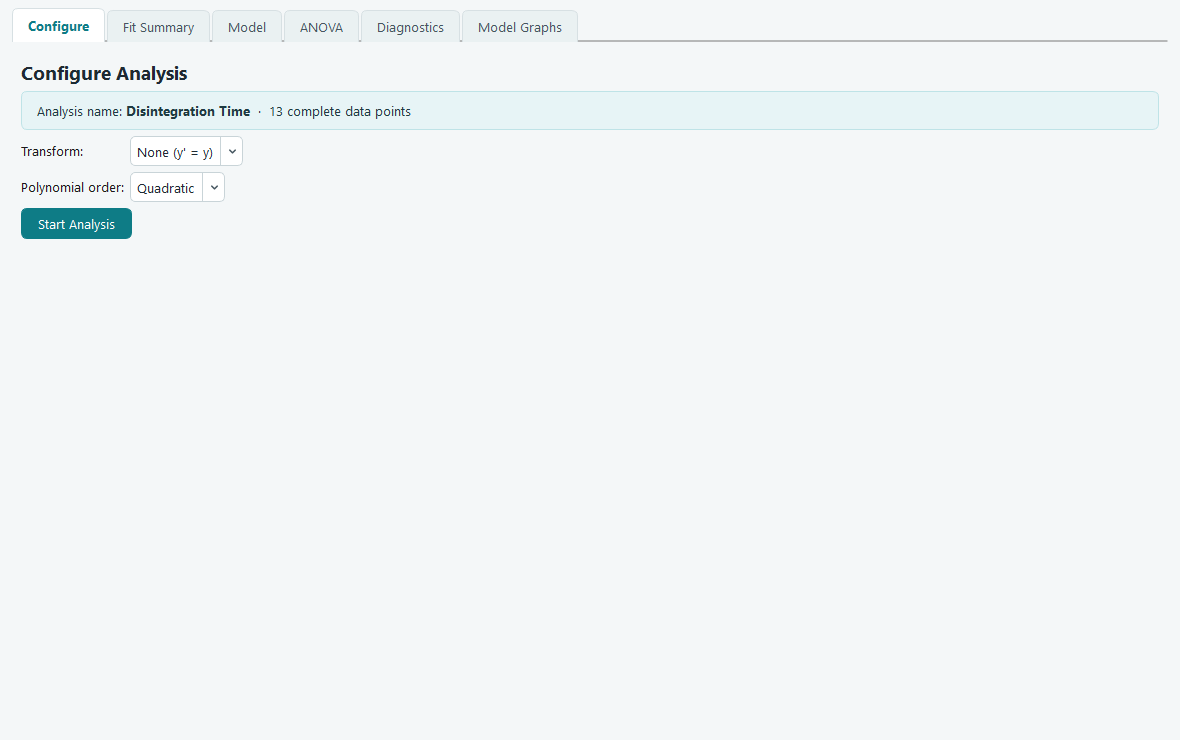
Transform decides whether the response is analysed as measured or on a changed
scale. The default is None (y' = y), which analyses the numbers exactly as you typed
them. Leave it there unless the residuals tell you otherwise. The Diagnostics tab draws a Box-Cox
plot that recommends a transform when one would help, so the usual path is to fit once with None,
read the diagnostics, and come back only if the plot points elsewhere.
Polynomial order chooses how many kinds of term the model may contain: Linear (main effects only), 2FI (main effects plus two factor interactions), Quadratic (adds squared terms, so the surface can curve), or Cubic. When the page first opens, the software has already looked at your data and preselected the order it suggests, so in most cases you can accept it and move on.
Press Start Analysis. The fit runs, and the page moves you to the Fit Summary tab. The button then reports that the analysis is complete and greys out. If you later change the transform or the order, the button wakes up again, because the results on screen no longer match your choices until you re-run.
Fit Summary: which model does the data support?
You do not have to guess the order. Fit Summary fits Linear, 2FI, Quadratic and Cubic in turn and lays out, side by side, how each one performs. Its job is to steer you toward the simplest model the data can justify.
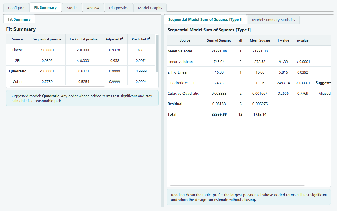
The left table has one row per order with four numbers to read:
- Sequential p-value. This asks whether the terms that order adds to the one below it are worth keeping. A small value (below 0.05) means the extra terms explain real variation, so climbing to this order paid off. A large value means the added terms are noise.
- Lack of Fit p-value. This compares the model against the pure error measured from your replicate runs. Here a large value is the good one: it says the model does not miss any real pattern. A small value (below 0.05) warns that something systematic is escaping the model.
- Adjusted R-squared and Predicted R-squared. Both run toward 1. Adjusted R-squared rewards fit but charges for every extra term. Predicted R-squared, built from the PRESS statistic, estimates how well the model forecasts runs it has not seen. You want both high and close to each other.
The right panel shows the working. The Sequential Model Sum of Squares table (Type I) reads top to bottom as a staircase: Mean vs Total, then Linear vs Mean, 2FI vs Linear, Quadratic vs 2FI, and so on, each line testing only what its order adds. The Model Summary Statistics table lists the standard deviation, the three R-squared measures and PRESS for each order together, so you can compare candidates at a glance.
How the software picks a suggestion
One row is flagged Suggested. The choice is not a guess; it is the documented Whitcomb score, the same rule practitioners use by hand. For each order the software forms a score from three ingredients:
- a sequential-p factor that is 1 when the added terms are significant and shrinks as that p-value climbs above 0.05,
- a lack-of-fit factor that is 1 when lack of fit is comfortably non-significant and shrinks as that p-value drops below 0.10,
- and the model's Predicted or Adjusted R-squared.
Multiply the three together and the order with the best score wins. Because the first factor is set to zero for any order the design cannot fully estimate, an aliased model can never be suggested. Aliased rows are labelled as such so you understand why they were skipped. When the Predicted and Adjusted scores disagree, both rows are flagged and the software defaults to the higher order.
Model: choose the exact terms
An order like Quadratic is really a bundle of terms. The Model tab opens that bundle so you can add or drop individual terms and watch the fit respond. This is where you trim a term that is not earning its place, or force one in that theory says belongs.
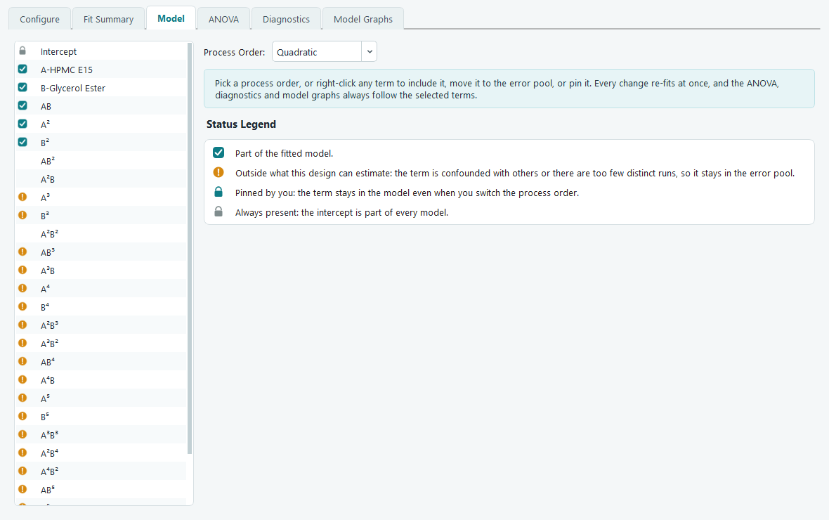
The Process Order picker on the right is the quick way to set the whole term set: Design Model (the model this design was built to support), Mean, Linear, 2FI, Quadratic, and higher orders where the design has room for them. Choosing one rewrites the term list. The moment you touch an individual term, the picker switches to Modified to show the set is now hand-built.
The icon beside each term is its status:
| Icon | Meaning |
|---|---|
| Teal check | The term is part of the fitted model. |
| Amber exclamation | The design cannot estimate this term: it is confounded with others, or there are too few distinct runs. It stays in the error pool. |
| Teal padlock | You pinned it. It stays in the model even when you change the process order. |
| Grey padlock | The intercept, which is part of every model. |
Right-click any term (or a selection of them) for Include in Model, Move to Error, or Pin Term. Every change re-fits at once, and the ANOVA, diagnostics and model graphs always follow the terms you have selected here.
ANOVA: read the verdict
With a model chosen, the ANOVA tab is where you decide whether to believe it. The analysis of variance splits the total variation in the response into the part the model explains and the part left over, then tests each piece.
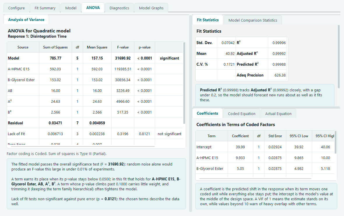
The main table lists a Model row, then one row per term, then Residual, Lack of Fit, Pure Error and the corrected total. Read it column by column:
- Sum of Squares and df are the variation attributed to each source and its degrees of freedom. Each model term uses one degree of freedom.
- Mean Square is the sum of squares divided by its df.
- F-value is the term's mean square over the residual mean square: how large the effect is compared with the noise.
- p-value is the chance of seeing an F that large if the term truly did nothing. The Model row is significant when its p-value is below 0.05. A term earns its place when its p-value stays below 0.05; a term whose p-value climbs past 0.10 carries little weight, and dropping it (keeping the family hierarchical) often tightens the model.
The Lack of Fit row is the one to check last. It compares the model's misses against the pure error from your replicate centre points. You want it not significant: a p-value above 0.05 means the chosen terms describe the data well. If it comes back significant, some real structure sits outside the model, and a higher order or a transform is worth trying. Beneath the table, the software restates the verdict in words, computed from this exact fit, so you are not left translating the numbers yourself.
Fit statistics: what good looks like
The Fit Statistics panel gathers the summary numbers for the chosen model. Here is how to read each one.
| Statistic | What it is | What good looks like |
|---|---|---|
| Std. Dev. | Root of the residual mean square, in the response's own units. | Small next to the mean. |
| Mean | Average of the response over the runs. | Context for the others. |
| C.V. % | The standard deviation as a percent of the mean. | Lower is better; the noise is a small slice of the signal. |
| R-squared | Fraction of variation the model explains. | Close to 1. |
| Adjusted R-squared | R-squared with a penalty for every term. | Close to 1 and close to R-squared. |
| Predicted R-squared | From PRESS: how well it predicts left-out runs. | Close to 1, and within about 0.2 of Adjusted R-squared. |
| Adeq Precision | A signal-to-noise ratio for the fitted surface. | Above 4. |
A gap of more than about 0.2 between Adjusted and Predicted R-squared is a hint to look for an outlier, a block effect, or too many terms. The Model Comparison Statistics tab adds PRESS, the log-likelihood, BIC and AICc for weighing one candidate model against another; for those scores, smaller values win.
Coefficients, confidence intervals and VIF
The Coefficients table gives the fitted value of every term along with a 95% confidence interval and a variance inflation factor. A coefficient is the predicted shift in the response when its term moves one coded unit while everything else holds still; the intercept is the model's value at the centre of the design space. If a coefficient's confidence interval straddles zero, that term is not clearly different from zero. The VIF measures how much a term overlaps the others: a VIF of 1 means the estimate stands on its own, while values past 10 warn of heavy overlap. For an orthogonal design like this central composite, the interaction and main-effect VIFs sit at or near 1.
The two equations, and when to use each
Once the model is fit, the software writes it out twice. Both describe the same surface; they differ only in the units their factors take.
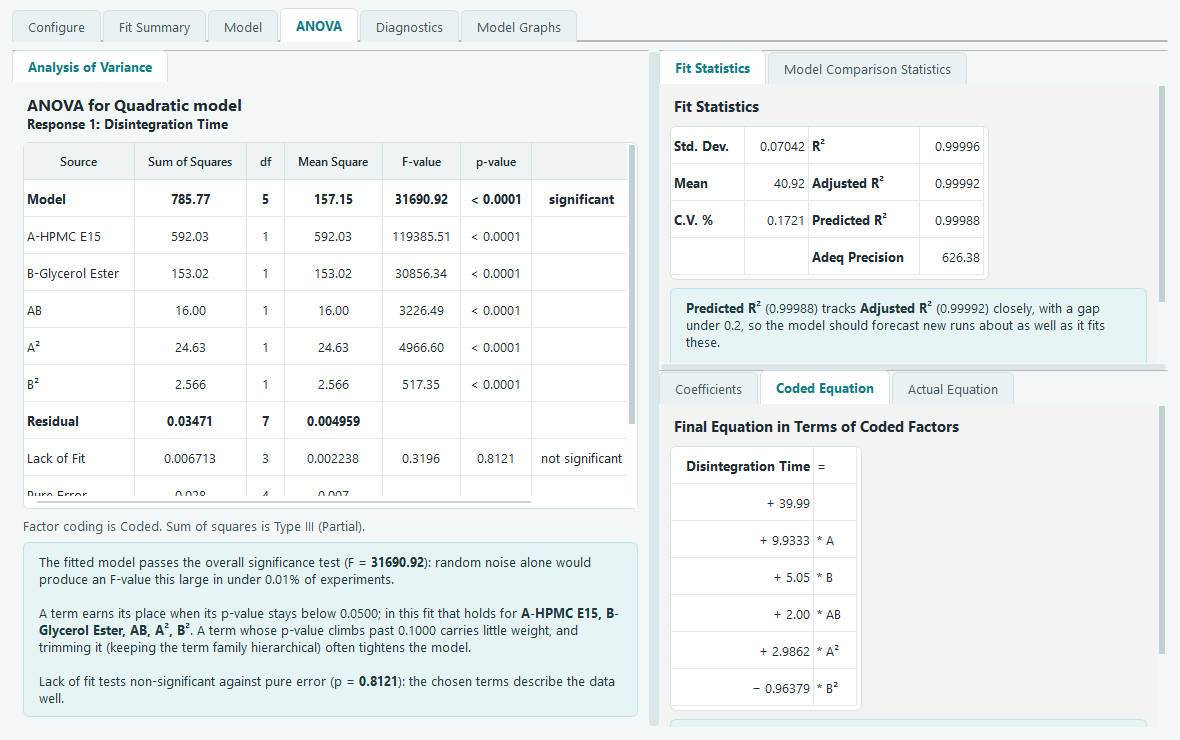
Use the coded equation to compare importance. Because every factor is on the same -1 to +1 scale, the size of each coefficient tells you directly which factors carry the most weight. This is the form to read when you want to know what matters.
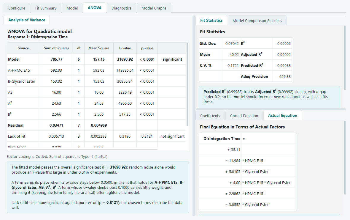
Use the actual equation to predict. It takes factor values in their original units, for example HPMC E15 in % w/v, so you can enter real settings and read off a predicted response. Do not compare its coefficient sizes: the unit scaling inflates or shrinks them, so a big coefficient there can simply mean a factor measured in small numbers. Judge importance from the coded equation, and predict from the actual one.
With a model you trust, move on to check its residuals before you rely on it.