Diagnostics
The ANOVA tells you the model fits. Diagnostics tell you whether you are allowed to believe it. This tab checks the assumptions behind every p-value, so you catch a bad run or a wrong model before it reaches a report.
Diagnostics is the fifth tab on an analysis page, after Configure, Fit Summary, Model and ANOVA. It exists because least squares makes promises: the residuals are random, they have the same spread everywhere, and they follow a normal distribution. When those promises hold, the ANOVA is trustworthy. When they do not, a small p-value can be an illusion. Every plot here is one way of asking whether the promises hold for your data.
The tab is a grid of four resizable plot panes plus a Report table. Each pane has its own sub-tabs, so a lot of graphs live in a small space. Every point is coloured by its response value, from blue at the low end to red at the high end, which helps you see whether trouble is concentrated in the big or the small results. Hover any point to read its exact numbers. All of this is recomputed from your data the moment you press Start Analysis on the Configure tab.
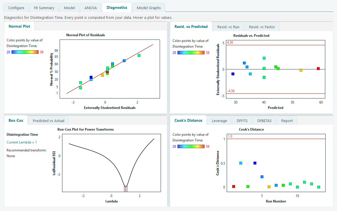
Normal plot of residuals
This is the first assumption to check. The plot puts the externally studentized residuals on the horizontal axis and their normal probability on the vertical axis, with the vertical scale stretched so that a normal distribution comes out as a straight line. A reference line is drawn for you to compare against.
- Points close to the straight line. The residuals are near normal. This is what you want, and minor wobble at the ends is normal and not a concern.
- An S shape, or a clear bend. The residuals are skewed rather than symmetric. That usually means the response should be transformed. Read the Box-Cox plot below before you do anything.
- One point stranded far out to the left or right. A possible outlier. Note its colour and go find it in the Report table.
Residuals versus predicted, run and factor
The second pane holds three related plots, each with the externally studentized residual on the vertical axis and a zero line through the middle. Red control lines mark the outlier limit: any point beyond them is worth a look. The limit is a Bonferroni corrected t value, computed from your design rather than fixed in advance. It takes account of the number of runs and the residual degrees of freedom, so the cutoff fits the size of your experiment instead of being one blanket number.
- Residuals versus Predicted. You want a shapeless, even band of points around zero. A funnel or megaphone, where the spread grows as the predicted value grows, means the variance is not constant. That breaks an assumption and is the classic sign that a transform is needed.
- Residuals versus Run. The points are joined in run order. A trend, a drift, or a step partway through means something changed over the course of the experiment, a warming room or an ageing reagent for example. This is exactly why the run order is randomised, so such drift shows up here instead of masquerading as a factor effect.
- Residuals versus Factor. Pick a factor from the box. A curved pattern here means that factor has curvature the model did not capture, which is a hint to raise the polynomial order on Configure.
Box-Cox plot for a transform
When the plots above suggest a transform, the Box-Cox plot tells you which one. It refits the model at many powers of the response and plots the natural log of the residual sum of squares against the power, called lambda. The lowest point on the curve is the transform the data likes best.
Three markers make it readable. A blue line sits at your current lambda, which is the transform set on the Configure tab. Out of the box the response is untransformed, so the current lambda is 1. A green line sits at the best lambda, the value at the bottom of the curve. Two red lines mark a 95 percent confidence interval around the best value. The text panel on the left states the current lambda and a plain recommendation, such as Natural Log or Square Root or None.
How to read it: if the blue current line falls inside the red interval, no transform is needed and the recommendation reads None. If the blue line sits outside the interval, the response would benefit from the transform named in the panel. Box-Cox needs every response value to be positive, so if a response contains a zero or a negative number the plot explains that instead of drawing a curve.
Predicted versus actual
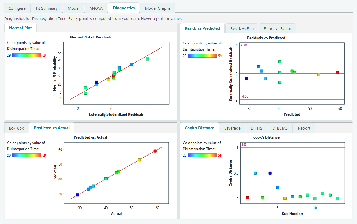
This plot, shared with the Box-Cox pane, is the simplest honesty check in the tab. It puts your measured values on the horizontal axis and the model's predictions on the vertical axis, with a diagonal reference line for a perfect fit. Points hugging the diagonal mean the model predicts what you actually saw. A point that sits well off the line is one the model struggles with, and its colour tells you at once whether the misses are among the high or the low results.
Influence: who is steering the model
A model is fitted to all the runs at once, but not every run pulls with equal force. The fourth pane holds four influence measures, each plotted against run number with a threshold line that the software draws for you. A point past its line is not automatically wrong; it is simply a run with enough sway that you should know it is there.
| Measure | What it asks | Line the software draws |
|---|---|---|
| Cook's Distance | How much every prediction would shift if this one run were removed. | A flag at 1.0. |
| Leverage | How unusual this run's factor settings are, on their own, before the response is even looked at. | Twice the average leverage, 2p divided by n, capped at 1, where p is the number of model terms and n the number of runs. |
| DFFITS | How far this run's own prediction moves when the run is left out, in standard errors. | Plus and minus 2 times the square root of p divided by n. |
| DFBETAS | How much one chosen coefficient changes when this run is left out. Pick the term from the box. | Plus and minus 2 divided by the square root of n. |
Leverage deserves a word. In the worked face-centred central composite design, the runs sitting on the edges of the factor ranges naturally carry more leverage than the five centre points, because their settings are further from the middle. High leverage on its own is a feature of a good design, not a fault. It only becomes a worry when a high leverage run also has a large residual, because then it is both influential and poorly fitted.
What to do when a point is flagged
A flag is a question, not a verdict. Work through it in this order.
- Check the data first. Open the run sheet and look at that run. A transposed digit, a wrong unit, a value typed into the wrong response: these account for most flagged points and are fixed in seconds.
- Ask what happened at the bench. If the number is typed correctly, think back to that run. A spill, a mislabelled sample or an instrument that misbehaved is a real reason to treat the run with suspicion.
- Repeat the run if you can. The cleanest resolution to a doubtful point is to run it again and see which value is real.
- Only then consider setting it aside, and say so plainly in your Notes. Removing a run changes every result on every tab.
The Report table
The Report sub-tab lays out every per run diagnostic as one row per run, so you can scan the whole design at once and match a flagged plot point to its actual numbers. The columns are Run Order, Actual Value, Predicted Value, Residual, Leverage, Internally Studentized, Externally Studentized, Cook's Distance, DFFITS and Std Order. Two columns highlight problems in red for you: the externally studentized residual when it passes the outlier limit, and DFFITS when it passes its threshold. Those red cells are your shortlist of runs to investigate.
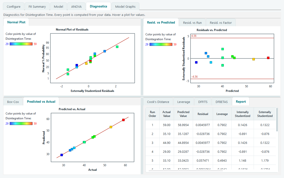
When the plots are clean, the normal plot is straight, the residuals are an even band, no point is flagged and Box-Cox recommends None, you can trust the ANOVA and move on. The next tab draws the model you have just validated.