Screening with a factorial
Early in a project you often have a long list of factors and no idea which ones actually move the response. Screening is the cheap first pass that sorts them out. You test all of them together in a small number of runs, then keep only the few that matter. This tutorial walks that pass from end to end with a two-level factorial.
Why screen first
Studying every factor in full detail is expensive. If you have six candidate factors, mapping each one carefully could cost dozens of runs before you even know whether half of them do anything. A screen turns the question around. Instead of asking "what is the exact shape of each effect", it asks "which factors have any effect worth chasing". Once you know the vital few, you can spend your remaining runs on those and drop the rest.
A two-level factorial is built for this. Every factor is set to just a low and a high value, so each factor costs very little, and you can pack many of them into one compact plan. The price of that economy is resolution: in a small plan some effects get tangled together, and part of the skill is choosing a plan where the tangles do not hide what you care about.
The example
Say you are developing a film coating for a tablet and six things might affect how fast the tablet disintegrates: the HPMC E15 level, the glycerol ester (plasticiser) level, the coating temperature, the spray rate, the pan speed and the curing time. You measure one response, Disintegration Time in seconds. The goal here is not to optimise anything yet. It is to find out which two or three of these six factors are worth a proper study.
Step by step
-
From the welcome screen choose New Design, then pick Regular Two-Level under the Factorial family. The panel on the right explains what the design is for and how to read the grid you are about to see.
-
You now choose the size of the plan on a grid. Each cell is one possible design: how many factors across the top, how many runs down the side. The cell colours are the important part. Green cells reach Resolution V or better, so main effects and two-factor interactions all stay readable. Amber cells are Resolution IV, which keeps main effects clean but lets two-factor interactions overlap each other. Red cells are Resolution III, the cheapest option, where main effects themselves can be confounded with interactions.
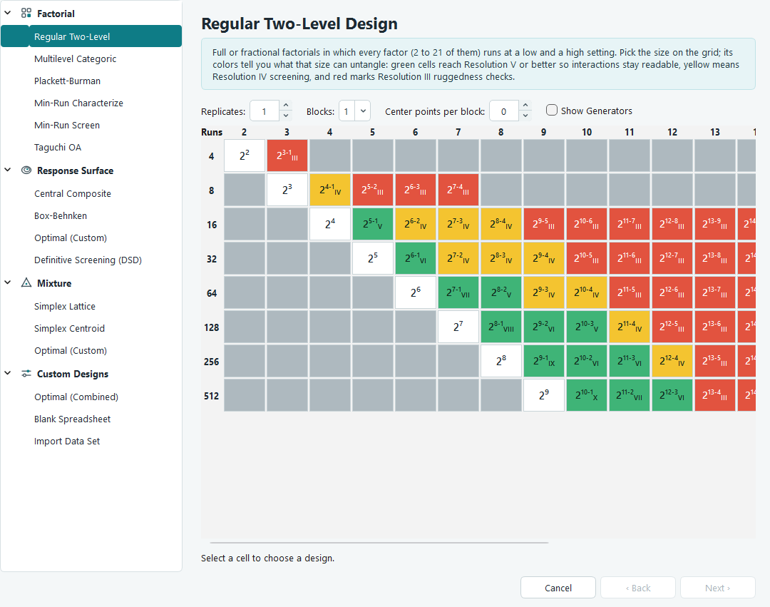
The two-level grid. Pick a cell, then read the line underneath: it names the design, the run count and the resolution in the same colour as the cell. For six factors, the 16-run cell is a good screening choice. The software marks it a quarter fraction at Resolution IV (amber): every main effect comes out clean, which is exactly what a screen needs. Tick Show Generators if you want to see the defining relation that spells out which effects share a column. You can also set replicates, blocks and centre points here, but for a first screen the defaults are fine.
Resolution is a trade. A greener cell answers more questions but costs more runs. Screening usually lives in the amber band on purpose: you accept that interactions are blurred together, because at this stage you only want to know which factors matter, not how they combine. -
Press Next and name your factors. Give each one a label, its units, and the low and high settings you will actually run. The letter (A, B, and so on) stays as the factor's short name, and the label you type is what appears everywhere else, so a run sheet column reads like
A:HPMC E15 (% w/v). -
On the last page, define your response. Here that is Disintegration Time in seconds. Leave Randomize run order ticked, then press Finish to build the run sheet.
Why the order is scrambled. The Run column is the order in which to perform the experiments, and it is deliberately randomised. If anything drifts while you work, a warming room or an ageing reagent, randomising stops that drift from lining up with any one factor and being mistaken for its effect. -
Perform the runs in the order shown and type each measured Disintegration Time into the response column. You can paste a whole column from a spreadsheet with Ctrl + V, and undo any slip with Ctrl + Z.
-
Open the response under Analysis in the navigation tree. The tabs run left to right in the order you use them: Configure, Fit Summary, Model, ANOVA, Diagnostics, Model Graphs. Start on Fit Summary. It compares the models the design can support and flags the one the data backs, marking anything the plan cannot separate as aliased. For a screen the answer is usually a main-effects model, sometimes a two-factor interaction model if a couple of interactions stand out.
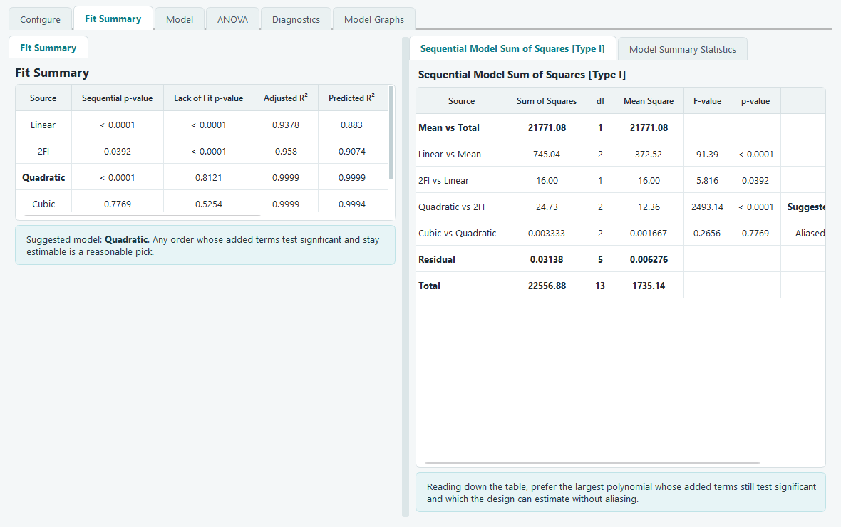
Fit Summary suggests a model and marks the terms the design can and cannot estimate cleanly. About these screenshots. The analysis pictures on this page come from the response surface example used elsewhere in this guide, which studies HPMC E15 and glycerol ester in detail. The analysis screens look and behave the same whatever design produced the data, so read them for the layout, not for the exact numbers. -
Move to the ANOVA tab. This is where a screen pays off. The table lists every term with its F-value and p-value, and the plain-language note underneath tells you which terms carry weight. A term earns its place when its p-value stays below 0.0500. Those significant main effects are your vital few. Any factor whose p-value climbs past 0.1000 is probably doing nothing, and you can drop it.
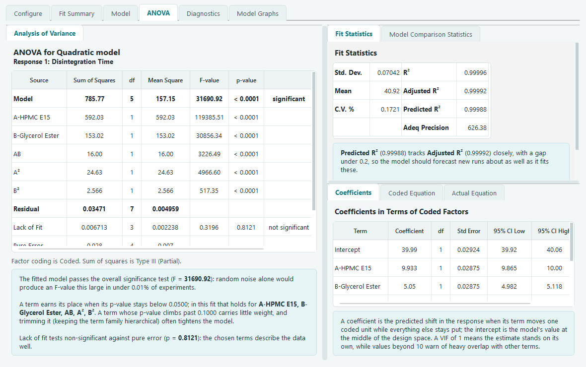
ANOVA, with the significance verdict written out below the table. The terms that stay under 0.0500 are the factors worth keeping. -
If two of the surviving factors both matter, check whether they interact. Open Model Graphs and choose the interaction plot. Two lines that stay parallel mean the factors act independently. Lines that cross or fan apart mean the effect of one factor depends on the setting of the other, which is worth knowing before you plan the next stage.
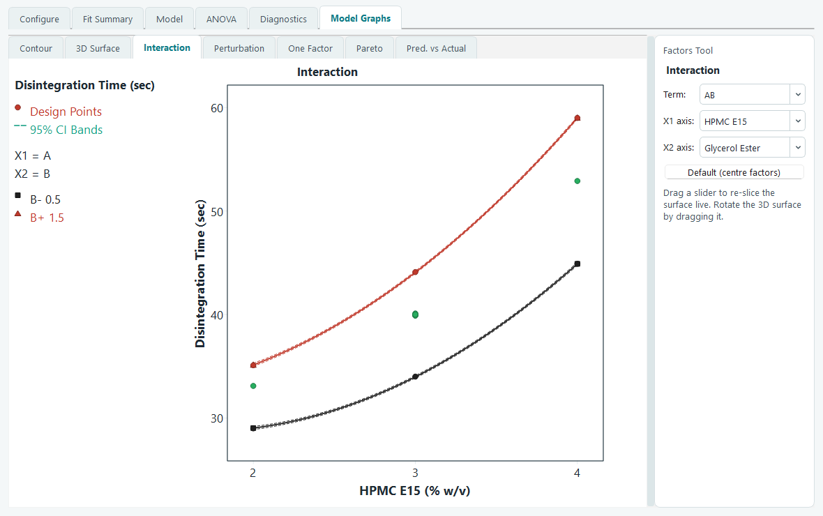
An interaction plot. Non-parallel lines say the two factors do not act independently.
Reading the result
At the end of the screen you have a short list. In the coating example, suppose the ANOVA shows that HPMC E15 and glycerol ester dominate the disintegration time while temperature, spray rate, pan speed and curing time all test non-significant. That is the whole point of screening: four factors have been cleared away, and you can now focus every remaining run on the two that count.
What to do next
Once you know the vital few, you change goal. Screening was about which factors; the next stage is about how they behave.
- If a couple of factors clearly matter and you now want the shape of the response and an optimum, move to a response surface design on just those factors. That is exactly the path the main tutorial takes: it studies HPMC E15 (2 to 4 % w/v) and glycerol ester (0.5 to 1.5 % w/v) with a face-centred central composite design. See Response surface, start to finish.
- If you have three to five survivors and want to characterise how they interact before optimising, a full two-level factorial or a Min-Run Characterize design keeps every interaction readable. See Factorial designs.
- Before you spend money on the next set of runs, it is worth checking the plan on the evaluation screen, and confirming a promising setting with a confirmation run.