Custom designs and import
The Custom Designs family is for the cases that do not fit a standard template: one experiment that studies a recipe and a process together, an empty sheet you plan by hand, or a set of results you already have and want to analyse. This page covers all three.
Optimal (Combined)
Sometimes the answer depends on both the recipe and the way you make it. The blend of ingredients matters, and so does a process choice such as the mixer you use or whether a coating step is on or off. Running a separate mixture study and a separate process study wastes runs and hides the interactions between the two. The Optimal (Combined) design puts them in one experiment. It crosses the mixture model with the process factors and asks a Fedorov exchange to pick the most informative combined runs inside the run budget you allow.
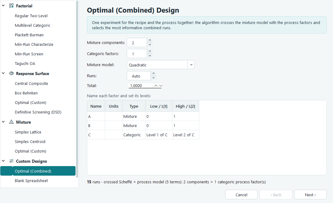
On the configuration page you set the number of mixture components (2 to 8) and the number of process factors, which you enter in the categoric factors field. A combined design needs at least one process factor to cross with, so that field starts at one. In the factor table the component rows are marked Mixture and run from 0 to the mixture total, and the process rows are marked Categoric with two levels each. Pick a mixture model, linear or quadratic, and the software crosses it with the process factors. Leave the run count on Auto to get the number of model terms plus ten, or type a fixed number if your budget is set. The line under the table tells you the run count and the term count as you change the options.
Blank Spreadsheet
Not every experiment is planned inside the software. You may already have trials you ran by hand, or historical batches from the plant, or a plan a colleague gave you on paper. The Blank Spreadsheet gives you an empty run sheet with the factors and responses you name, and nothing filled in. You type or paste every setting and every result yourself.
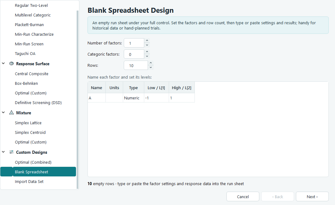
Set the number of factors (1 to 20) and the number of rows you need. Each factor can be numeric, with a low and a high value, or categoric, with two levels; the categoric factors field controls how many of the rows are categoric. Move to the next page to name your responses. When you press Finish you get a run sheet of the size you asked for, all cells empty, ready for you to enter the data. From that point the sheet behaves like any other design: you can paste a whole column from a spreadsheet and undo with Ctrl + Z.
Import Data Set
Import Data Set reads a table you paste from the clipboard and turns it into a design you can analyse. It is the fastest way to bring in results that were recorded somewhere else. The screen is a single page: paste your data, tidy the rows, tell the software what each column is, then press Finish.
-
Copy the whole block of data from the source, in Excel, a text file, or anywhere that copies tab or comma separated text. A header row of names at the top is fine.
-
Click Paste from Clipboard. The software splits the text into rows, and splits each row on tabs if it finds any, otherwise on commas. If the first row looks like text labels sitting above numeric data, it treats that row as a header and drops it, so the labels are not mistaken for a run.
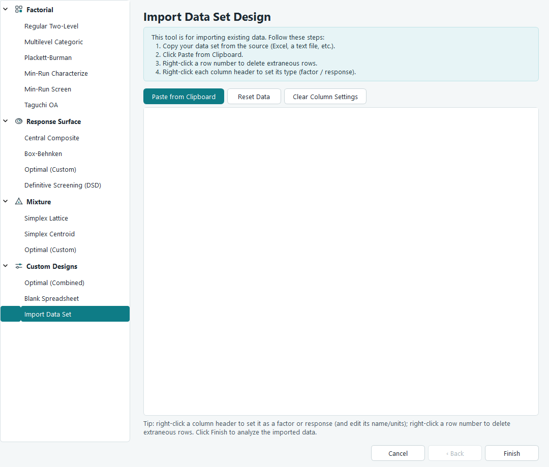
Pasted data. Every column starts unassigned and shows (set type) until you give it a role. -
Delete anything that is not a run. Right-click a row number and choose Delete Row, or select several rows and right-click to delete them together. Blank separator lines, subtotals and stray notes should all go. You can also insert a row if you need to.
-
Set the role of each column. Right-click a column header and open Set Column Type, then choose Numeric Factor, Categoric Factor, Response or Ignore. To set several columns at once, click their headers with Ctrl or Shift first, then right-click and apply the type to all of them.
-
Name each column. Right-click a single header and choose Edit Info to type its name and units. This is worth doing, because the header names you pasted are not carried over automatically.
-
Click Finish. The imported table opens as a normal design workspace, ready to analyse.
Two buttons help you start over without leaving the page. Reset Data empties the whole table so you can paste a different block. Clear Column Settings keeps the data but returns every column to unassigned, which is useful when you mislabelled the roles and want a clean slate.
What the software works out, and what it cannot
The importer reads structure, not meaning. It is worth knowing exactly where the line falls so you are not surprised by the result.
| The software works this out for you | You have to tell it this |
|---|---|
| Whether the block is tab or comma separated, and where the rows and columns fall. | Which columns are factors and which are responses. Every column starts with no role. |
| Whether the top line is a header of labels, which it then drops. | The name and units of each column. Defaults are the plain factor letters A, B and so on, and R1, R2 for responses, until you set names with Edit Info. |
| The range of a numeric factor, taken as the lowest and highest value in that column. | Whether a column of numbers is really a numeric factor or a categoric one written as codes. Set it as Categoric if the numbers are labels. |
| The levels of a categoric factor, taken as the distinct text values in that column. | The order of the runs. Rows are kept exactly as pasted; there is no randomisation. |
Analysing imported data
An imported data set analyses exactly like a design the software built for you. You can fit a model, read the ANOVA, check the residuals and draw the model graphs, all in the usual Analysis tabs. There is one honest caveat. A built design places its runs on purpose so that the model terms can be told apart cleanly. Your imported runs were chosen for other reasons, so they may not have that property.
This shows up under Information, in the Evaluation screen. For an imported set it may report high variance inflation, which means two terms move together and their effects are hard to separate; it may list terms the design cannot estimate at all; and it may show uneven leverage, where a single run has too much pull on the fit. None of that is a fault in the software. It is telling you the truth about data that was not collected to a plan. Read Evaluating a design to understand each measure, and treat a weak evaluation as a reason to be careful with the conclusions, not as an error to fix.