Mixture designs
Reach for a mixture design when the factors are the parts of one recipe and the response depends on the proportions, not the amounts. This page explains why a recipe needs its own kind of design and covers the three mixture types the software builds: Simplex Lattice, Simplex Centroid and Optimal (Custom).
What makes a mixture different
In an ordinary experiment you can set each factor on its own. Temperature does not care what the pressure is. A recipe is not like that. Its components are proportions of one whole, so they are tied together by a single rule: they have to add up to a fixed total. If a tablet blend is filler, binder and lubricant, and you raise the binder, something else has to come down to make room. You can never move one component while holding the rest still, because the total is not allowed to change.
That one constraint changes everything about the design. The response you care about is usually the blend, not the batch size. A film at 30% plasticiser behaves the same whether you mix one gram or one kilogram, so what the experiment varies is the set of proportions, and those proportions always sum to one (or to whatever batch total you set).
Why a factorial does not work here
Picture three components on three ordinary axes, each running from 0 to 1. A factorial or a response surface design would put points at the corners of a cube: all-low, all-high, and every mix in between. Almost none of those corners is a legal recipe. The point where all three components are at their maximum does not exist, because three things at 100% each cannot share one batch. The only points that obey the sum rule lie on a flat slice cutting across that cube.
That slice is the simplex, and it is where every mixture design lives. Its shape depends on how many components you have:
| Components | Shape of the design space | The corners are |
|---|---|---|
| 2 | A line segment | All of A, or all of B |
| 3 | A triangle | The three pure components |
| 4 | A tetrahedron | The four pure components |
| q | A q-cornered simplex | Each single pure component |
The corners of the simplex are the pure components. The edges are two-part blends. The interior holds the blends that use every component at once. A mixture design is simply a sensible set of points spread across this simplex, and the three types below spread them in different ways.
How a mixture model is fitted
The sum constraint also reshapes the model. An ordinary polynomial starts with an intercept, a plain constant sitting under everything else. In a mixture that constant cannot be separated from the component terms: because the components always add to the same total, any constant could be hidden inside the linear terms and nobody could tell the difference. The intercept and the component terms are aliased with one another.
There are two equivalent ways to resolve this. The classical Scheffe form drops the intercept and keeps one linear coefficient for every component. OptiGein Design uses the other one, known as the slack variable form: it keeps the intercept and drops whichever single component term the sum constraint has made redundant. That term is reported as Aliased on the Fit Summary and Model tabs. This is the software telling you the design cannot estimate it separately, not a sign that something has gone wrong.
Because the intercept is kept, a coefficient in the OptiGein equation is not the response you would expect from that pure component, which is how a Scheffe linear coefficient is usually read. Read the coefficients the way you read them everywhere else in the software: as the shift in the response as that component increases, with the dropped component taking up the balance. If you want the value for a pure component, do not do the algebra by hand. Use Point Prediction, set that component to its maximum and the others to their minimums, and read the number off directly.
Squared terms such as A² do not appear in a mixture model. The sum rule lets you rewrite any squared term using the linear and cross product terms, so it carries no new information and is left out. What remains are the component terms and one cross product term for each pair of components.
| Mixture model | Terms | Count for q components |
|---|---|---|
| Linear | One per component, one of which is aliased away | q |
| Quadratic | Components plus every pair | q + q(q−1)/2 |
Setting a minimum and a maximum for a component
Real recipes rarely allow a component to run from nothing to everything. The design screen lets you give each component a Low and a High, and the software respects them.
A minimum simply shrinks the blend region. If a preservative must always be at least 2 percent, every blend the software builds carries at least 2 percent of it, and the remaining 98 percent is what the design explores. The runs still add up to the total, and each component can still reach as high as the others allow: with everything else held at its own minimum, a component reaches its own minimum plus whatever is left over.
A maximum is different. If a maximum actually bites, meaning the component could otherwise have reached higher, it slices a corner off the blend region and leaves a shape that a lattice or a centroid cannot cover with its regular pattern of points. Rather than quietly building blends that break the limit you typed, Simplex Lattice and Simplex Centroid stop and tell you. The Optimal (Custom) mixture design has no such restriction, because it chooses its runs from a pool of candidate blends and simply ignores the ones that break a bound.
The cross-product coefficients are the useful part. A positive coefficient on the A×B term means the two components together do better than either one alone, a synergy. A negative one means they work against each other. That is exactly the question a formulator wants a mixture experiment to answer.
Simplex Lattice
A simplex lattice spreads points evenly over the whole simplex on a regular grid. You choose the number of components, from 2 to 12, and a lattice degree written as m. The degree sets the spacing: each component is placed at the proportions 0, 1/m, 2/m and so on up to 1, and the design uses every combination of those levels that still adds up to the total. A higher degree samples the edges and faces more finely and supports a higher-order blending model, so match m to the model you intend to fit: 1 for a linear blend, 2 for a quadratic one, and higher if you expect a more curved response.
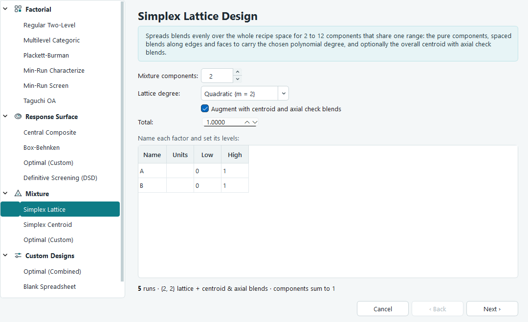
For three components at degree 2 that gives six runs: the three pure components at the corners and the three fifty-fifty blends at the edge midpoints. The number of grid points grows with both the component count and the degree, so the software caps a lattice at 1000 runs and asks you to lower the degree if you ask for more.
A plain lattice keeps all of its points on the outside of the simplex, on the corners, edges and faces. That is fine for fitting the model but it leaves the middle of the space unchecked. The augment option, which is on by default, fixes this. It adds the overall centroid, the blend that uses every component in equal parts, and one axial check blend per component sitting partway between the centroid and each corner. Those extra points let you see whether the model that fits the boundary also predicts the interior well, which is where real formulations usually live.
Simplex Centroid
A simplex centroid is built around equal-parts blends rather than a grid. For q components, from 3 to 10, it runs every non-empty combination of components mixed in equal parts. That means each pure component on its own, every fifty-fifty pair, every equal three-way blend, and so on, all the way down to the single overall centroid that mixes all q components equally. The run count is a clean 2q−1, so three components give seven runs and four give fifteen.
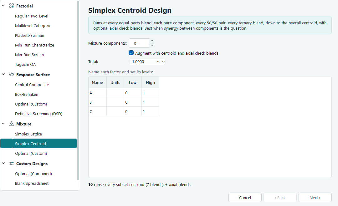
Because it visits blends of every size, the centroid design is the natural choice when the question is about interaction between components: does a three-way blend behave like the average of its pairs, or does something new happen when all three are present at once. Like the lattice, it offers the same augment option, which adds one axial check blend per component so the interior of the simplex is not left to the model alone.
Optimal (Custom)
The two designs above place their points by a fixed rule. An optimal mixture places them by search. You tell the software how many components you have, from 2 to 10, whether you want a linear or a quadratic Scheffe model, and how many runs your budget allows. It then works through a large pool of candidate blends across the simplex and, using a D-optimal exchange, keeps the subset of runs that measures your chosen model most precisely.
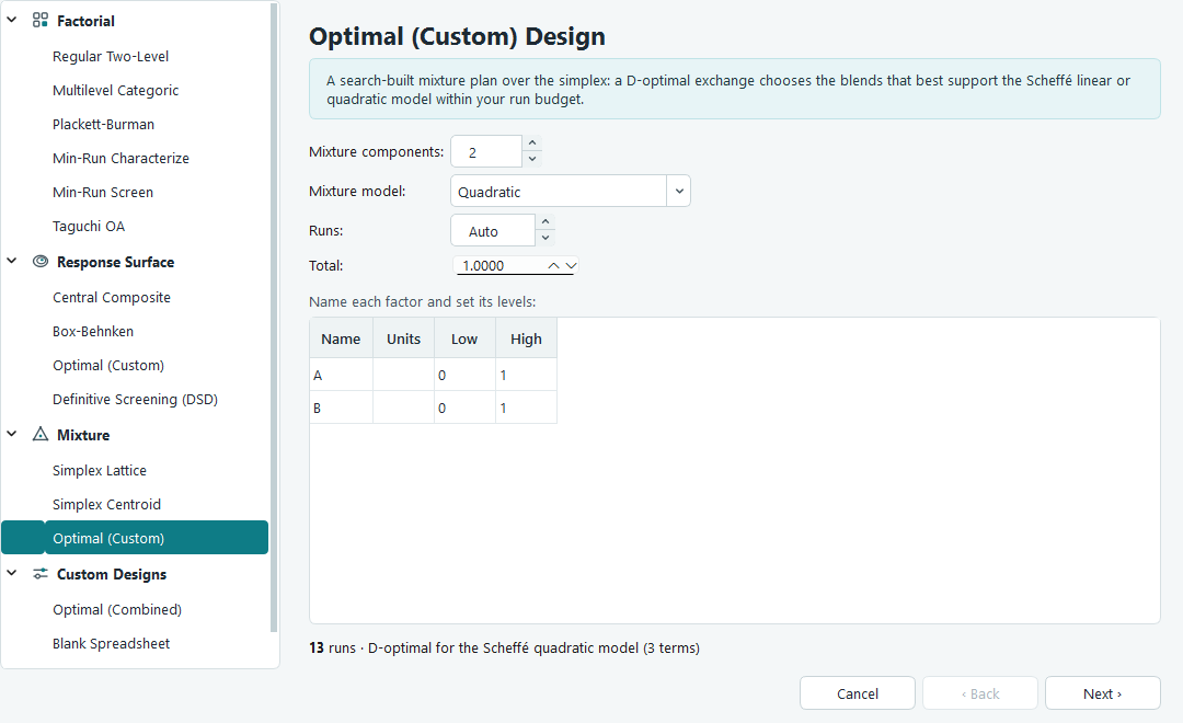
This is the design to use when a lattice or centroid does not fit your situation: you have an awkward number of components, a tight run budget, or you simply want the smallest sensible design for a known model. If you leave the run count blank the software proposes a default of the number of model terms plus ten, which leaves a few spare runs to estimate error. You can never ask for fewer runs than the model has terms; the design screen tells you the minimum as you change the model.
Reading the run sheet
However the points are chosen, each mixture run reaches the run sheet as real component amounts. The
software multiplies each proportion by the total you set, so if your total is 100 mg the columns read
in milligrams and every row still sums to 100. Component columns carry the same header style as any
other factor, the design letter followed by the name you gave it, so a column might read
A:Lactose (mg). Fill in the response columns exactly as you would for any other design,
then move to the Analysis branch to fit the Scheffe model.
| Design | Components | Places points by | Best when |
|---|---|---|---|
| Simplex Lattice | 2 to 12 | An even grid of degree m | You want an evenly spread model-fitting design |
| Simplex Centroid | 3 to 10 | Equal-parts blends of every subset | Interaction between components is the question |
| Optimal (Custom) | 2 to 10 | A D-optimal search on a run budget | Runs are limited or the component count is awkward |
What to read next
- A mixture experiment walks one recipe from an empty screen to a recommended blend.
- Custom designs and import covers the combined mixture and process design.
- Fit summary, model and ANOVA explains how the fitted model is judged.