Evaluating a design
Evaluation looks at a design before you run it. It cannot tell you the answer to your experiment, because there are no results yet. What it can tell you is whether the design you are about to run is strong enough to give you a clear answer, while it is still cheap to fix.
You open Evaluation from the Information branch of the navigation pane. It studies the pattern of factor settings in the run sheet, nothing else, so it works the moment a design is built and long before any response is measured. The page assumes a model, then asks two questions about it: can this design estimate every term in the model, and how precisely will it do so. Weak spots show up as large numbers in a few key columns, and the fixes are usually simple: add a few runs, add centre points, or fit a smaller model.
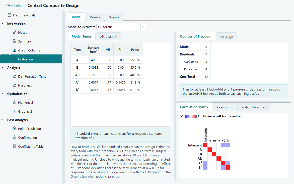
The page has three tabs across the top: Model, Results and Graphs. The Model tab is the working area with every table. The Results tab is the same information as a plain, printable report. The Graphs tab holds the fraction of design space curve.
Choosing the model to evaluate
Precision is always relative to a model, so the first thing you do is pick one. The drop-down at the top left offers main effects only (linear), two-factor interactions (2FI), and quadratic. The design cannot care what you eventually fit, but the evaluation numbers can change a lot with the model, so evaluate the model you actually intend to analyse. For the response surface example the quadratic model is the right choice, since a central composite design exists precisely to fit curvature.
Degrees of freedom
Degrees of freedom are your experiment's budget. Every run buys you one, and each part of the analysis spends some. The table splits the total into the pieces that matter.
| Line | What it counts |
|---|---|
| Model | Terms the model spends, one per coefficient other than the intercept. More terms need more runs. |
| Residuals | What is left over to estimate error and to test the model. This is where your safety margin lives. |
| Lack of Fit | The part of the residual that checks whether the model shape is right. It needs runs at settings that are not centre points. |
| Pure Error | The part that measures pure noise, from genuine replicates such as repeated centre points. |
| Corr Total | The whole budget, which is the number of runs minus one. |
For the example, the quadratic model spends 5 degrees of freedom on the terms A, B, AB, A squared and B squared. That leaves 7 residual degrees of freedom out of a corrected total of 12. The 5 centre points give 4 pure-error degrees of freedom, and the remaining 3 go to lack of fit.
Leverage and average leverage
Leverage measures how much one run pulls the fitted surface toward its own result. A leverage near 1 means the model is forced to pass almost exactly through that point, so a single bad measurement there bends the whole surface and you never see it in the residuals. The table lists the leverage of every run, its space type, and an average at the bottom. The average leverage is simply the number of coefficients divided by the number of runs, so a lower average means the design spreads its effort more evenly. Where you see a leverage close to 1, replicate that run or perform it with extra care.
Per-term precision: standard error, VIF and Ri squared
The Model Terms table has one row per model term and tells you how well each will be estimated. Because there are no results yet, precision is quoted for a response with a standard deviation of 1, so the numbers compare terms and designs rather than predict real units.
| Column | How to read it |
|---|---|
| Standard Error | The uncertainty on that term's coefficient. Similar values down the column mean the design estimates every term with even precision, which is what you want. |
| VIF | Variance inflation factor. It says how much a term's variance is enlarged because it is correlated with the other terms. A VIF of 1 is ideal: the term is estimated independently. Above 10 signals strong multicollinearity, and that term's coefficient will be hard to trust. |
| Ri squared | How well the other terms predict this one. Close to 0 is good and means the term stands apart from the rest of the model. VIF and Ri squared measure the same problem from two angles. |
| Power | Your chance of catching a real effect. See below. |
A high VIF is usually a sign that two effects move together in your run sheet, so the design cannot pull them apart. Orthogonal designs, such as a clean factorial, show a VIF of 1 on every term. Central composite and other response surface designs carry mild correlation between the squared terms, which is normal and expected.
Power: the chance of detecting an effect
Power answers the practical question, if this factor really does matter, will my experiment notice. The column reports the probability of declaring a term significant at the 0.05 level when its true effect is 2 standard deviations across the factor's range. A power of 90 percent means that nine times out of ten a real effect of that size would be flagged; 40 percent means you would miss it more often than not. Low power comes from too few runs relative to the number of terms, and the cure is more runs.
Design quality measures and prediction variance
Below the per-term table, the design quality measures score the design as a whole. The most useful ones describe prediction variance, that is, how uncertain the model's predicted mean is at a point in the factor space, again for a response standard deviation of 1.
| Measure | Meaning |
|---|---|
| Maximum, average and minimum prediction variance | The spread of prediction uncertainty across the region. A small gap between maximum and minimum means the design predicts about equally well everywhere. |
| G efficiency | How close the worst-case prediction variance comes to the ideal. Higher is better, quoted as a percentage. |
| Scaled D-optimality | An overall score for how precisely the whole set of coefficients is estimated. Smaller is better. |
| Determinant and trace of the inverse information matrix | Two more overall precision scores. Smaller values mean tighter coefficients. |
| Condition number | How near the design is to being unable to separate its terms. Large values warn of numerical trouble and heavy correlation. |
The fraction of design space curve
Open the Graphs tab for the fraction of design space, or FDS, curve. It is the single best picture of how evenly a response surface design predicts. Read it left to right: the horizontal axis is the fraction of the design space, from none of it to all of it, and the vertical axis is the largest standard error of the predicted mean over that fraction. A point at 0.8 on the curve tells you the error you can expect over the best-covered 80 percent of the region.
You want a curve that is both low and flat. Low means predictions are precise; flat means they are just as precise near the edges as they are in the middle, with no corner of the space left vague. A curve that climbs steeply on the right is warning you that predictions get unreliable toward the extremes, which often means the design needs more runs out at the boundary.
When the numbers look bad
Evaluation is only worth running if you act on it. A few patterns and their usual fixes:
| What you see | What to do |
|---|---|
| VIF well above 10, or a high condition number | Terms are tangled together. Add runs to break the correlation, or fit a smaller model that drops the terms you do not truly need. |
| Low power on effects you care about | Add runs. Power rises as the residual budget grows. |
| Zero or tiny lack-of-fit or pure-error degrees of freedom | Add centre points for pure error, and add non-centre runs so lack of fit has something to test. |
| An FDS curve that is high or rises sharply at the right | Add runs, especially near the edges of the region, or reduce the model order. |
| A run with leverage near 1 | Replicate that run, or perform it with extra care so one measurement cannot bend the fit. |
Reducing the model is the fix people forget. A design that struggles with a full quadratic can be perfectly strong for a two-factor-interaction model, so switch the drop-down and look again before you commit to extra runs. Every change you make to the design updates the page the next time you open it, so you can try a fix and see the numbers move before you spend anything in the lab.