A mixture experiment
Some experiments are about a recipe, not a machine. You have three ingredients that must add up to the whole blend, and you want to know how their proportions change the result. This walk through builds a three component blend, enters the results, fits the mixture model, and reads the surface, using a small tablet formulation as the example.
When the ingredients are the experiment
Suppose you are formulating a tablet filler from three excipients: lactose, microcrystalline cellulose and maize starch. Together they make up 100% of the blend, and you want to know how their proportions affect the disintegration time. This is a mixture problem, and it behaves differently from a factorial or a response surface.
The difference is the constraint. In a factorial you can turn one factor up while everything else stays put. In a blend you cannot: if you raise lactose from 30% to 40%, that extra 10% has to come out of the other two ingredients. The proportions are not free to move on their own, they always sum to the total. Because of that, a mixture design does not put the ingredients on a square grid. It spreads the blends across a triangle whose corners are the pure components, and it fits a model that respects the sum.
Build the design
A simplex lattice is the natural first choice. It places runs at the pure components, at evenly spaced blends along the edges of the triangle, and, when you ask for it, at the centre and a few check blends inside. That set of blends is exactly what the mixture model needs.
-
From the welcome screen choose New Design, open the Mixture
family and select Simplex Lattice. The panel on the right explains what the
design covers before you commit to it.
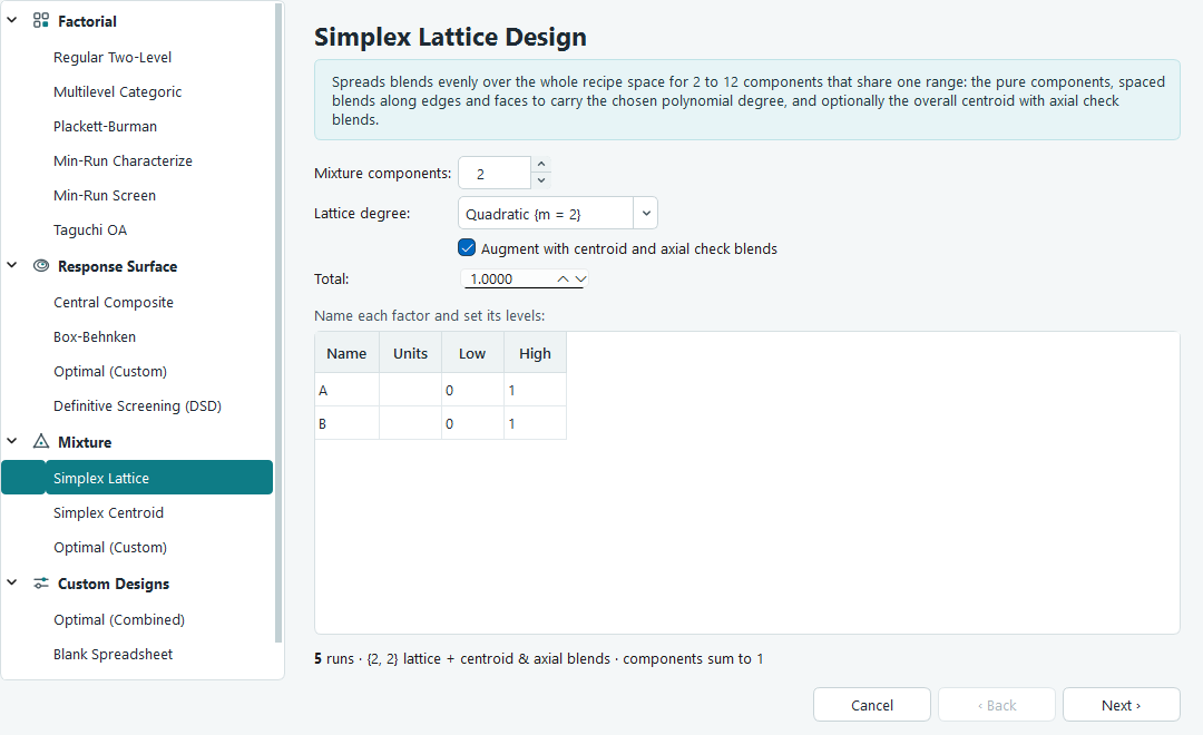
The Simplex Lattice page. The run count on the right updates as you change the component count, the degree and the augmentation. - Set Mixture components to 3. Simplex lattice supports 2 to 12 components.
- Set the Lattice degree to Quadratic {m = 2}. The degree controls how many blends sit along each edge, and therefore which model the design can support. Quadratic is the usual working choice: it lets curvature and two component blending show up.
- Leave Augment with centroid and axial check blends ticked. The plain lattice can fit the model but leaves nothing over to test it. The extra centre and axial blends give you runs to check the fit and estimate lack of fit.
- Set the Total to 100, since you are working in percent of the blend. The default total is 1, which suits fractions.
-
Give each component a name and a unit on the factor rows, for example
Lactose,MCCandMaize Starch, all in% w/w. Add one response,Disintegration Timeinsec. Press Finish to build the run sheet.
Internally the component letters are A, B and C, and the labels are the names you typed, so the
run sheet headers read A:Lactose (% w/w), B:MCC (% w/w) and
C:Maize Starch (% w/w).
The blends the software builds
A quadratic three component lattice has six blends: the three pure components and the three fifty to fifty edge blends. Augmentation adds the overall centroid and three axial check blends, for thirteen runs in all... no: ten runs in all. Here they are as percentages of the blend.
| Blend | A: Lactose | B: MCC | C: Maize Starch |
|---|---|---|---|
| Pure A | 100 | 0 | 0 |
| Pure B | 0 | 100 | 0 |
| Pure C | 0 | 0 | 100 |
| Edge A and B | 50 | 50 | 0 |
| Edge A and C | 50 | 0 | 50 |
| Edge B and C | 0 | 50 | 50 |
| Centroid | 33.3 | 33.3 | 33.3 |
| Axial toward A | 66.7 | 16.7 | 16.7 |
| Axial toward B | 16.7 | 66.7 | 16.7 |
| Axial toward C | 16.7 | 16.7 | 66.7 |
Every row sums to 100, which is the point. The pure components pin down the corners, the edge blends test how each pair works together, and the centroid and axial blends probe the middle where all three ingredients are present. The Run column randomises the order you should mix and measure them.
Enter your results
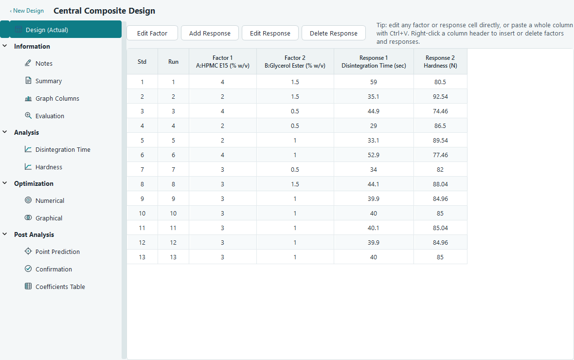
Run the blends, measure the disintegration time for each, and type the numbers into the response column of the run sheet. You can paste a whole column from a spreadsheet with Ctrl + V and undo a slip with Ctrl + Z.
Fit the mixture model
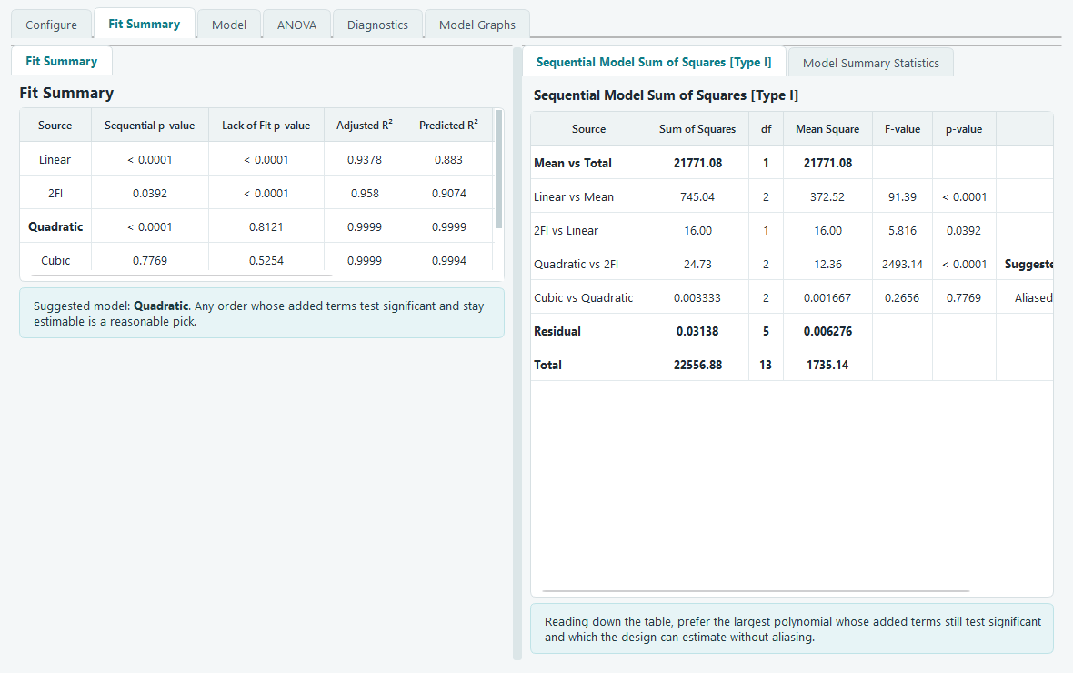
Open the response under Analysis and work along the tabs. The Fit Summary tab compares model orders and points you at the one the data supports. For a mixture the model carries a linear term for each component and, in the quadratic model, a cross term for each pair of components that captures how two ingredients blend. Because the components always add up to the same total, one component term cannot be estimated on its own and is reported as Aliased. That happens for every mixture design and costs you nothing: the predictions, the graphs and the optimum are unaffected. See how a mixture model is fitted for the reason.
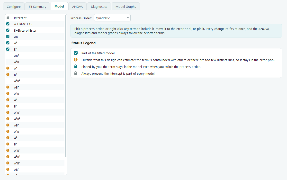
On the Model tab you can see and adjust the terms. This is also where the mixture constraint becomes visible in the software. Because the three components always add up to the total, one of them carries no information the other two do not already give: once you know lactose and MCC, maize starch is fixed. OptiGein detects that redundancy and marks the extra term as one this design cannot estimate, so it is left out of the fit rather than causing a divide by zero.
The ANOVA and equation panels behave as they do for any response. The coded and actual equations list the intercept and the estimable terms, and each table on the page carries a short plain language note under it that says what the numbers mean for your blend.
Read the surface
The Model Graphs tab draws the fitted response. It is worth being clear about what you see, because a mixture is often shown as a shaded triangle in textbooks. OptiGein draws the same rectangular contour and 3D surface it uses for a response surface design: two components go on the axes across their ranges, and the remaining component is held at a value you set with the sliders. It does not draw a triangular, three axis mixture plot.
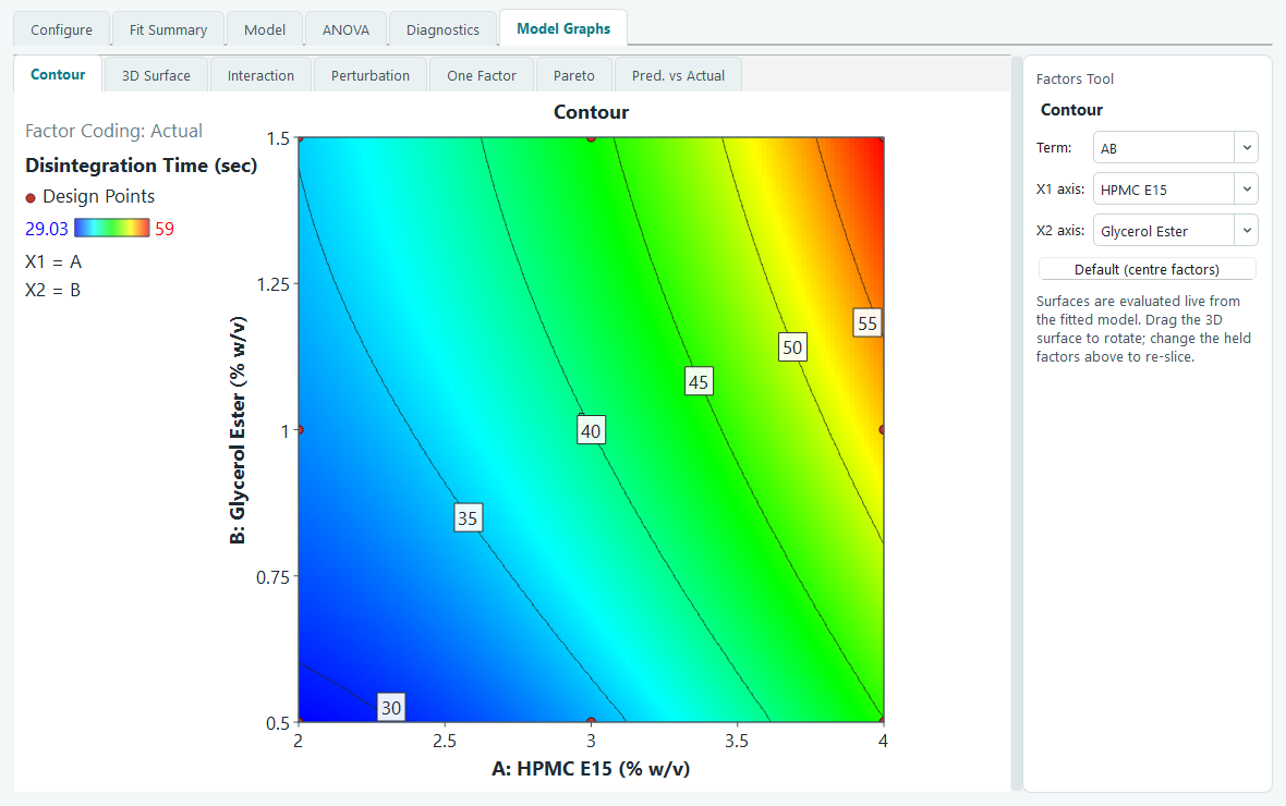
To read it as a recipe, remember the sum. If lactose is on the horizontal axis, MCC on the vertical axis and maize starch is held at, say, 20%, then only the blends where lactose plus MCC make up the other 80% are real recipes. Those lie along one diagonal line of the plot. Slide the held component to sweep that line across the triangle. When you want the response for one exact blend rather than a slice, use Point Prediction instead, which is not tied to a two component view.
Predict any blend, and the pure components
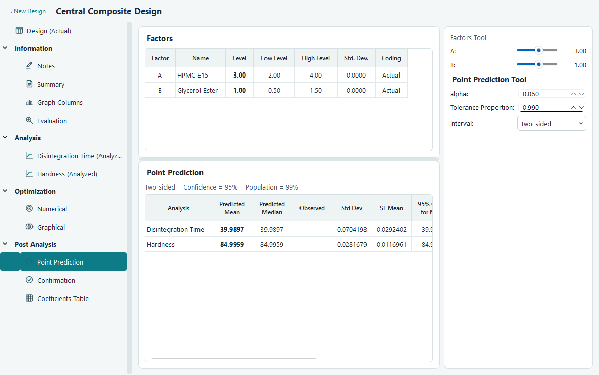
Under Post Analysis, open Point Prediction. Type the proportions of a blend you care about and the software returns the predicted disintegration time with a confidence interval. This is how you recover the pure component values that the classical coefficients would have given you: set one component to 100 and the other two to 0, and read the prediction. Do the same at any interior blend to compare recipes before you commit to a confirmation run.
What to read next
- Mixture designs for the simplex centroid and optimal mixture options, and when to prefer each.
- Fit summary, model and ANOVA for how the model tabs work in detail.
- Prediction and confirmation for Point Prediction and planning the runs that confirm your chosen blend.