Numerical optimization
Most experiments have more than one response, and the settings that are best for one are rarely best for another. Numerical optimization asks the fitted models a single question: which factor settings come closest to satisfying every goal at once. It answers by turning each goal into a desirability score, combining those scores, and searching for the highest total.
You reach this screen from the Optimization branch of the navigation pane, under Numerical. It has three tabs that you work through in order: Criteria, where you say what you want; Solutions, where the software lists the settings it found; and Graphs, where you see those settings in context.
Setting a goal for each factor and response
The Criteria tab lists your factors first, then your responses. Select one on the left and its editor appears on the right: a goal, a lower and upper limit, sometimes a target, weights, and an importance. Below the editor sits a picture of the desirability ramp for the current goal.
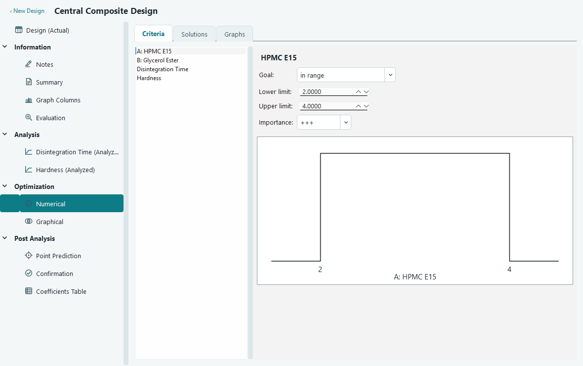
A goal is how you want a response to behave. Every response gets a desirability between 0 and 1: a 1 means the goal is fully met, a 0 means it is missed completely, and values in between measure how close you are.
| Goal | For a response | For a factor |
|---|---|---|
| none | Predict and report it, but leave it out of the search. | Not offered. |
| maximize | Score rises from 0 at the lower limit to 1 at the upper limit. | Pin the factor at its upper limit. |
| minimize | Score rises from 0 at the upper limit to 1 at the lower limit. | Pin the factor at its lower limit. |
| target | Score peaks at the target and falls to 0 at each limit. | Pin the factor at the target value. |
| in range | Any value between the limits scores 1, anything outside scores 0. | Let the search move the factor freely between the limits. |
| equal to | Not offered. | Pin the factor at the value. |
Factor goals do not add to the desirability. They shape where the search is allowed to look. Leave a factor in range and the optimizer is free to tune it; give it any other goal and you fix it, so you can ask questions like "what is the best hardness I can get if HPMC E15 is held at 3 % w/v".
For the worked example in these pages, a face-centred central composite design on A: HPMC E15 and B: Glycerol Ester, you might minimize Disintegration Time and aim Hardness at a target, while leaving both factors in range so the search can move them.
The lower and upper limits
The limits are the two ends of the ramp. For a response they default to the smallest and largest values you actually measured, which is a sensible starting range. Widen or narrow them to match what you care about. A result below the lower limit or above the upper limit scores 0 for that response, so the limits are also a hard boundary, not just a scale.
Weights and the shape of the ramp
A weight bends the ramp between a limit and the good end. With a weight of 1 the ramp is a straight line, so desirability grows evenly. A weight above 1 bends the ramp downward, so a result earns a high score only when it is close to the good limit. A weight below 1 bends it upward, so even a partial result already counts for a lot. There is a lower weight for the ramp on the low side and an upper weight for the high side; a target goal uses both, one for each slope.
You can set the weights in two ways. Type them into the Lower weight and Upper weight boxes, which accept values from 0.1 to 10, or drag the ramp directly. Each sloped part of the ramp has a small square handle at its middle. Drag a handle up to soften the ramp, which lowers the weight, or drag it down to make it stricter, which raises the weight. The boxes follow the handle, and the handle follows the boxes, so the two always agree.
Importance
Importance says how much a response counts against the others. You set it from one plus (+) to five pluses (+++++), with three pluses in the middle as the default. A response with five pluses pulls the search toward its own goal much harder than one with a single plus. Use it to break ties between responses that cannot all be satisfied perfectly.
How the scores combine
Each response gives one desirability. The software combines them into a single overall desirability, written as D, using an importance-weighted geometric mean. In plain terms, it multiplies the scores together, giving more say to the responses you marked as more important, then takes the matching root. Responses set to none are left out of this sum.
The Solutions table
Open the Solutions tab and the search runs. At the top, a Constraints table repeats every goal, limit, weight and importance you set, so the run is self-documenting. Press Find Solutions to run it again after any change.
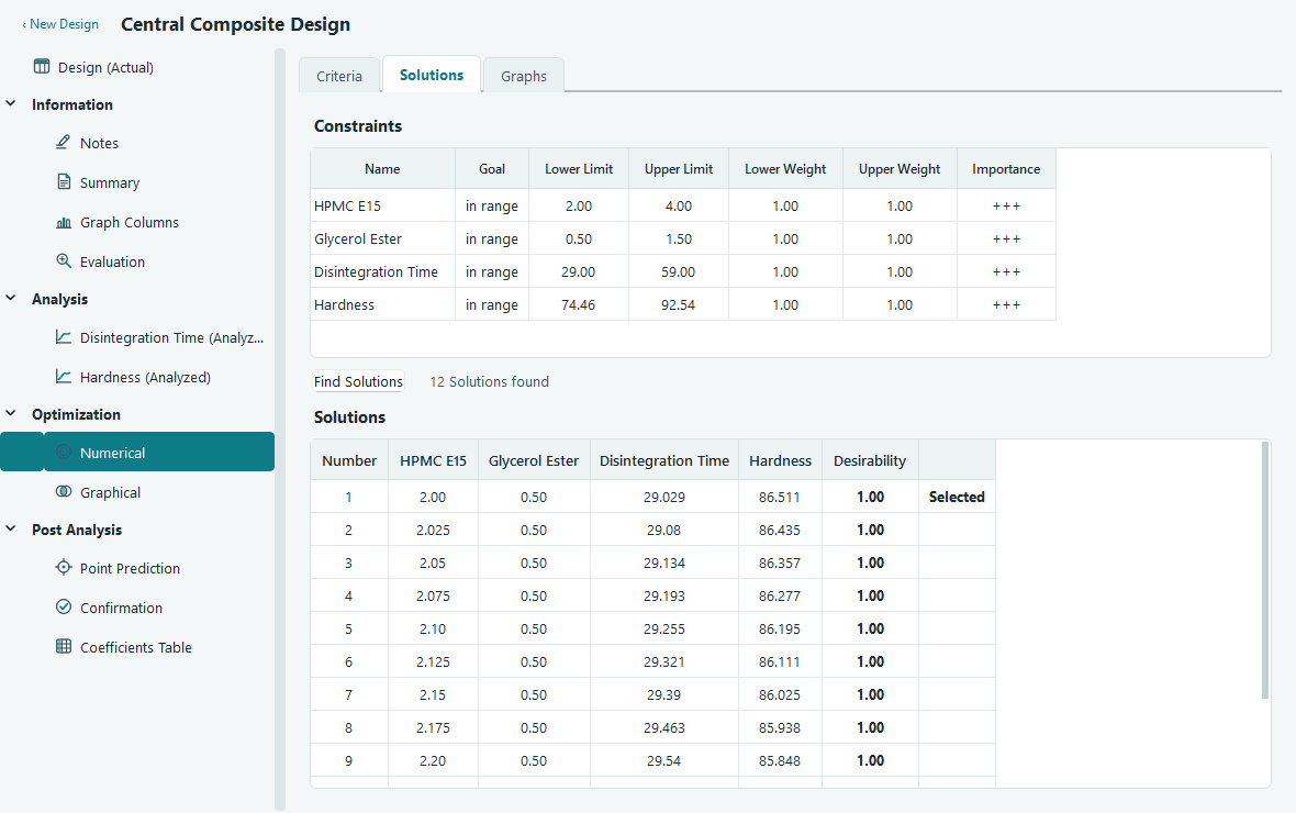
Each row is a set of factor settings the optimizer found, with the values it predicts for every response and the overall desirability for that row. The list is sorted with the highest desirability first, and the top row is marked Selected. The optimizer reports up to a dozen distinct settings, so you can compare near-equal options rather than trusting a single answer. Two rows with almost the same desirability may sit in very different places, and one may be far easier to run than the other.
The Graphs tab
Numbers in a table are hard to trust on their own. The Graphs tab draws the solution on the fitted surfaces so you can see how forgiving it is. Pick which surface to show with the Show list: the overall desirability, any single response, or All responses at once. On the right, the Factors Tool lets you choose which solution to plot and which two factors go on the axes.
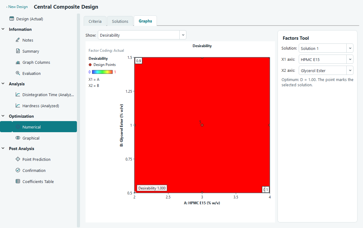
The desirability map is worth a look before you commit. A solution sitting on a steep slope or a narrow ridge is fragile: a small drift in a factor sends desirability down fast. A solution in a wide, gentle plateau is one you can hit in practice. The chosen point is marked on every plot, labelled with its overall desirability or its predicted value.
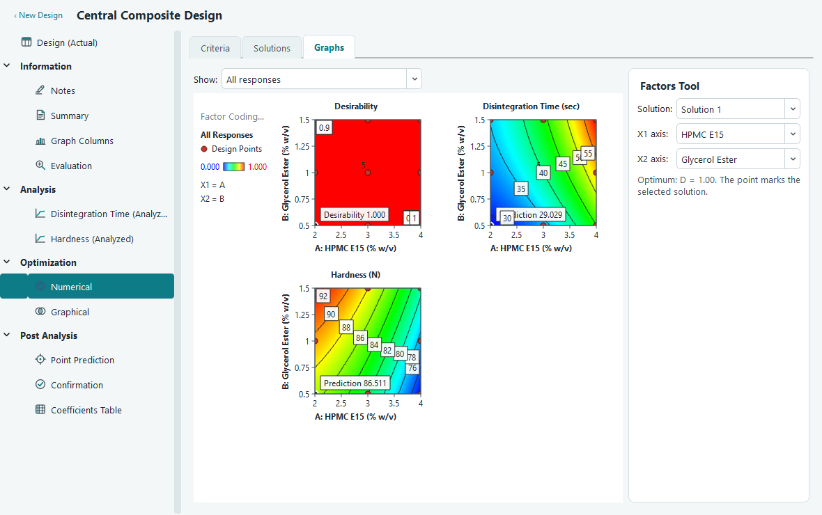
The All responses view puts the desirability map and one map per response into a single figure with a shared legend panel. The maps fill as many columns as your window allows and wrap onto new rows below when the width runs out, so every map stays a readable size whether you have two responses or ten, on a laptop screen or a large monitor. It is the clearest single picture of a solution, showing at a glance where each response lands as you move around the two factors. Because it is drawn as one figure, copying or exporting it gives you one combined image for a report.
Picking a solution and confirming it
The top solution is a suggestion, not a verdict. Choose the one you will actually run, then check it in the lab.
- On the Solutions tab, read across the rows and pick the settings that best fit your process. Click that row to select it. The Graphs tab and the Factors Tool follow your choice.
- Switch to the Graphs tab and confirm the point sits in a stable region of the desirability map, not on a steep edge.
- Note the factor settings from that row. Use Point Prediction under Post Analysis to read the predicted responses at those settings, together with their confidence and tolerance intervals.
- Run the chosen settings in the lab, then enter the measured responses on the Confirmation screen. It compares what you got against what the model predicted, so you can trust the optimum before you rely on it.