Response surface designs
These designs are for the stage after screening, when you already know which factors matter and you want the shape of the response, not just its direction. They let you fit curvature, find a peak or a valley, and settle on the best combination of settings.
Why you need more than two levels
A two-level design measures each factor at a low and a high setting only. Two points define a straight line, so a two-level design can tell you that a response rises or falls, but it cannot tell you that the response bends. Real processes bend all the time: a response climbs, flattens at an optimum, then falls again. To see that shape you have to test each factor at three or more settings, and you have to fit a model with squared terms. A model with squared terms is a response surface, and the four designs on this page are the ways OptiGein Design builds one.
Central composite
The central composite design is the usual first choice for two to ten numeric factors. It is built in three parts, and each part does a job:
- A factorial core. A two-level full or fractional factorial on the corners of the design space. This part estimates the main effects and the two-factor interactions, exactly as a screening design would.
- Axial points, also called star points. Two extra runs per factor, placed out along each factor axis with the other factors held at their centre. These runs are what make the squared terms estimable, so they are the reason the surface can curve.
- Centre replicates. Several runs with every factor at its middle setting. Repeating the centre gives a direct measure of pure experimental error and shows whether the middle of the surface sits where a flat model would predict.
Between the corners, the axial points and the centre, each factor ends up at five distinct settings, which is plenty to fit and check a quadratic model.
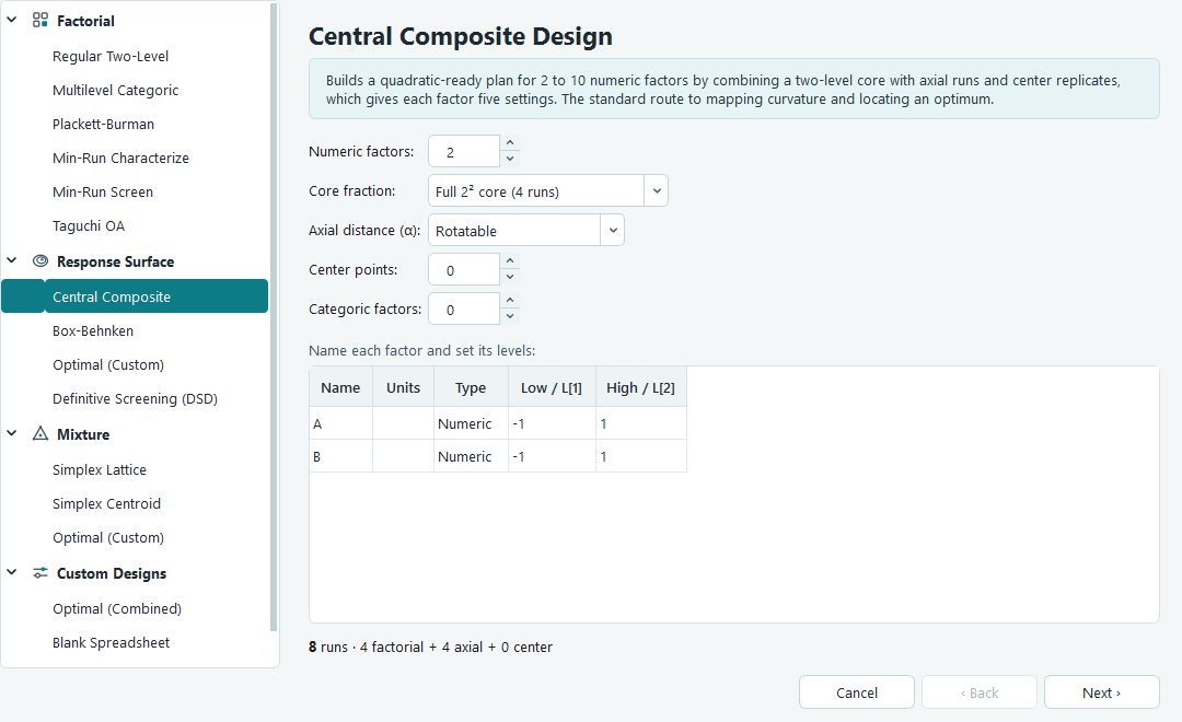
The axial distance, alpha
Alpha is how far out the star points sit, measured in coded units where the corners are at plus or minus one. The value of alpha decides whether those runs stay inside the factor ranges you typed or reach beyond them. The configuration page offers three choices.
| Choice | Axial distance | What it means physically |
|---|---|---|
| Rotatable | The fourth root of the number of factorial points, about 1.41 for two factors. | Prediction is equally precise in every direction at a given distance from the centre. The star points fall outside the low-to-high range you set, so each factor is run a little beyond its stated limits. |
| Spherical | The square root of the number of factors. | Every non-centre run sits on one sphere around the centre point. The star points again reach outside your ranges. |
| Face-centered (α = 1) | Exactly one. | The star points land on the faces of the cube, at the low or high level itself. No run ever leaves the ranges you set. Choose this when a setting past your limits is impossible, unsafe or too expensive to try. |
The worked example in this documentation is a face-centred central composite on two numeric factors, A: HPMC E15 from 2 to 4 % w/v and B: Glycerol Ester from 0.5 to 1.5 % w/v. It has 13 runs: four factorial corners, four axial points and five centre replicates. Because it is face-centred, every run stays inside 2 to 4 % w/v for HPMC and 0.5 to 1.5 % w/v for the ester, which is why you never see an out-of-range value on the run sheet.
The Core fraction field only matters once you have enough factors that a full factorial core would be wasteful. With many factors you can pick a fraction of the core, which trims the corner runs while keeping the axial and centre runs intact. With two or three factors the core is simply full.
Box-Behnken
Box-Behnken is a leaner three-level design for three to five numeric factors. Instead of corners and star points, its runs sit at the midpoints of the edges of the design cube, with the remaining factors held at their centre. Each numeric factor takes just three settings: low, middle and high.
The useful property is that no single run puts every factor at an extreme at the same time. Every run has at most two factors at a limit while the rest sit in the middle. If your corner combinations are the risky ones, all factors maxed together, a Box-Behnken design avoids them entirely. It also costs fewer runs than a full three-level factorial would.
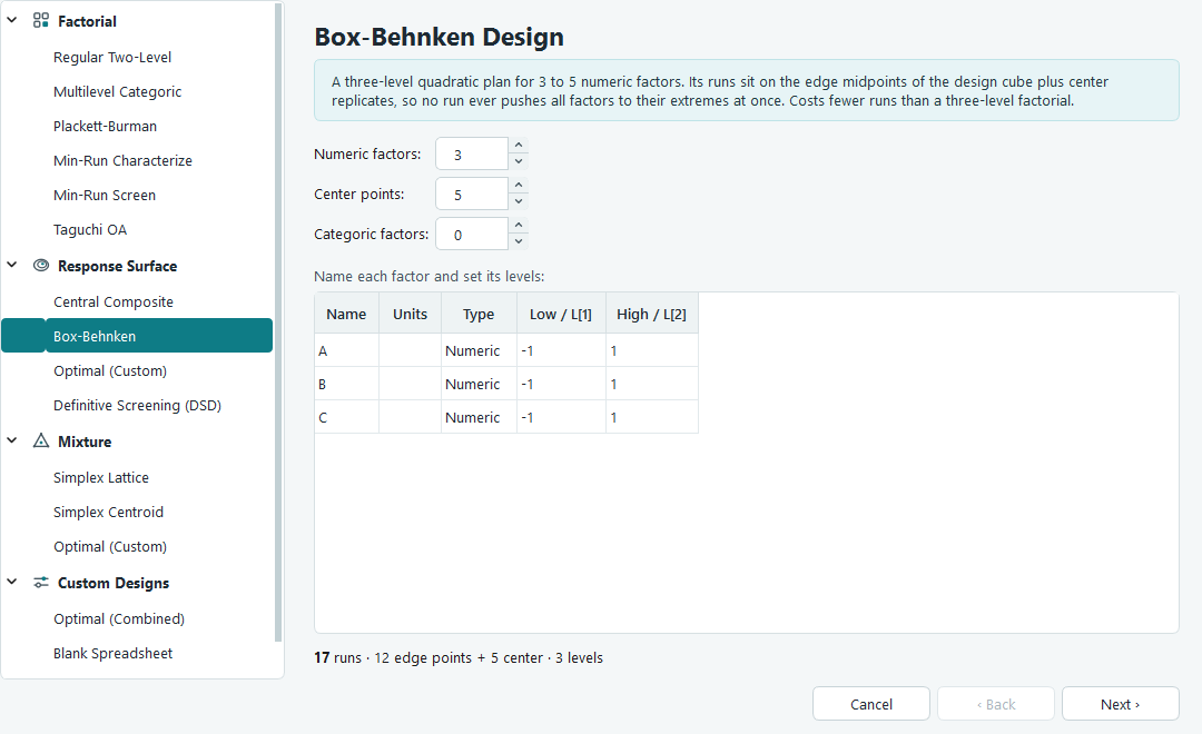
The number of edge runs grows with the number of factors: each pair of factors contributes four runs, so the total is four times the number of factor pairs. That works out to twelve runs for three factors, twenty-four for four and forty for five. On top of that, the design starts with five centre replicates by default, so a three-factor Box-Behnken is seventeen runs. You can change the centre count on the configuration page.
Optimal (Custom)
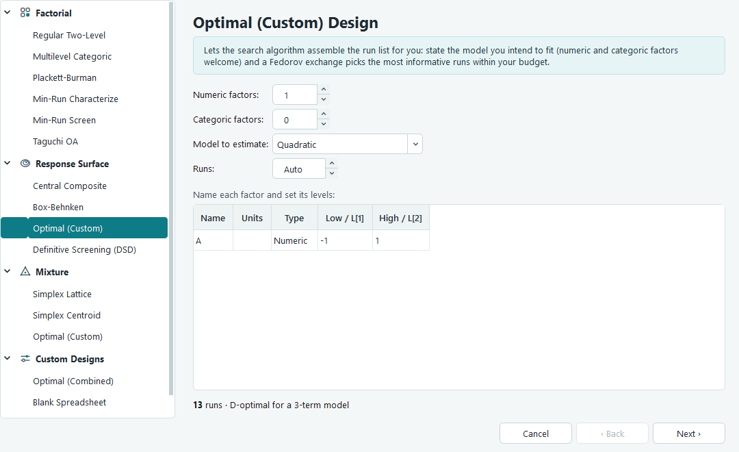
The two designs above have a fixed geometry. An optimal design does not: you tell the software what model you intend to fit and how many runs you can afford, and it chooses the runs for you. This is the design to use when your run budget is set in advance, when you mix numeric and categoric factors, or when the standard shapes do not fit your constraints.
On the configuration page you set the numeric factors, any two-level categoric factors, the model to estimate (main effects, two-factor interactions or quadratic) and the number of runs. Leave the run count on Auto and the software allocates the number of terms in your model plus ten, which leaves room to test for lack of fit and to estimate error. A Fedorov exchange algorithm then searches for the set of runs that measures your chosen model most precisely, swapping candidate runs in and out until the information it gathers stops improving.
Definitive screening
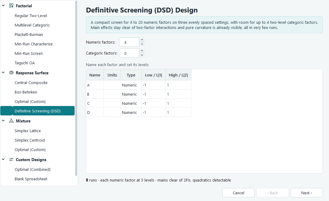
A definitive screening design, or DSD, sits between screening and response surface work. It is built for four to twenty numeric factors, each set at three evenly spaced levels, with room for up to four two-level categoric factors alongside them. Its appeal is how much it separates in very few runs, a little over twice the number of factors.
Two properties make it worth knowing. First, the main effects stay clear of the two-factor interactions, so a large main effect is never an interaction in disguise. Second, because every numeric factor runs at three levels, pure curvature is already visible, meaning you can see whether a factor bends the response before you commit to a full quadratic design. If only a few factors turn out to matter, a DSD often carries you far enough to model them without a second experiment.
What to read next
- Response surface, start to finish walks the face-centred central composite example from an empty screen to a recommended set of settings.
- Evaluating a design shows how to check a response surface design before you spend money on the runs.
- Which design do I need? compares the families side by side if you are still deciding.