Graphical optimization
Numerical optimization hands you a single best set of factor values. Graphical optimization shows you the whole neighbourhood around it: the range of settings where every response still meets its requirements. Use the two together and you get both the point and the room around it.
Why look at a picture
A single recommended point is easy to act on but tells you nothing about how forgiving it is. In the factory or the lab, factors drift. HPMC concentration is a little off, the room is warmer than usual, a batch of glycerol ester behaves slightly differently. What you really want to know is how much slack you have before a response falls out of specification.
The overlay plot answers that. You give each response a lower limit, an upper limit, or both. OptiGein Design then colours the factor space: yellow where every response stays inside all of its limits, grey where at least one response fails. The yellow patch is your operating window. A large patch means a robust process; a thin sliver means you have almost no margin, even if the numerical optimum sits inside it.
Set the limits
Open Optimization › Graphical in the navigation pane. It has two tabs, Criteria and Graphs. Start on Criteria. The list on the left shows every response you have already analysed. A response only appears here once it has a fitted model, so if one is missing, go back to its Analysis page and fit it first.
- Select a response in the list. The panel on the right names it and shows the range actually observed in your runs, so you have a sensible frame of reference for the numbers you are about to type.
- Type a value in Lower, in Upper, or in both. Leave a box empty
(it reads none) to say that side has no limit. For the worked example you might cap
Disintegration Time (sec) with an upper limit, because a tablet that takes too long to disintegrate
is no good, and give Hardness (N) a lower limit, because a tablet that is too soft will crumble.
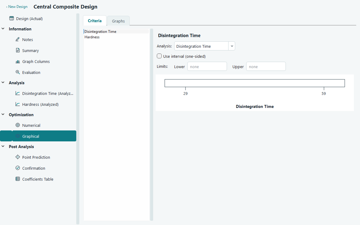
The Criteria tab. Each response gets its own lower and upper limits. The strip below shows the observed range with the chosen limits marked in red and the in-limit band shaded yellow. - Repeat for every response you care about. A response with no limits set does not constrain the plot at all, so only fill in the ones that matter.
The strip beneath the fields is a quick sanity check. It draws the response range your experiment
actually produced, marks your lower limit with a ≥ and your upper limit with a
≤, and shades the band between them yellow. If your limits sit right at the edge of the
observed range, or outside it, that is worth noticing before you read the overlay. If you type a lower
value above an upper value by mistake, the software quietly swaps them so the band still makes sense.
Read the overlay
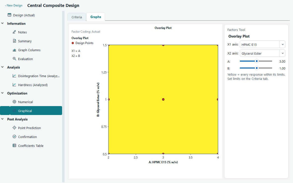
Switch to the Graphs tab. The overlay plot fills most of the page, with a Factors Tool panel on the right. Two axes carry two of your factors; every other factor is held fixed. For the two factor example, A: HPMC E15 and B: Glycerol Ester go straight onto the axes and nothing is held.
| What you see | What it means |
|---|---|
| Yellow region | Every response stays inside every limit you set. Any settings in here satisfy all of your requirements at once. |
| Grey region | At least one response fails at least one limit. You do not have to know which one; grey simply means out of bounds. |
| Coloured boundary curve | The line where one response is exactly equal to one of its limits. Cross it and that response tips over the edge. Each active limit gets its own colour, and the same colour keys the legend in the info panel on the left. |
| Red dots | Your actual design runs that lie in the plane being shown. They tell you whether your operating window is near real data or out in extrapolated territory. |
Each boundary curve carries a small label naming the response and the limit value, so you can tell at a glance which edge of the yellow region belongs to which requirement. The left panel lists the same limits with their colour swatches, the factors on the two axes, and the fixed value of any held factor.
When you have more than two factors
You can only draw two factors on the axes, so a design with three or more factors is shown as a slice: a flat cut through the factor space at fixed values of everything not on the axes. The Factors Tool panel gives you an X1 axis and X2 axis selector to choose which two factors to plot, and a slider for each remaining factor to set where the slice is taken. Its actual value updates beside the slider as you drag.
Moving a slider re-cuts the plane, and the yellow region grows, shrinks or shifts as you go. This is the point of graphical optimization with many factors: the operating window is not one fixed shape, it depends on where the held factors sit. Slide through them to find the combination that gives you the most generous window. The red design points also change, because only the runs that actually lie in the current slice are drawn.
When there is no yellow region
Sometimes the whole plot is grey. That is information, not a failure. It means no setting in the region you are looking at can satisfy all of your limits together. Before you give up, try these in order.
- Loosen a limit. Go back to the Criteria tab and relax the requirement that is hardest to meet. Even a small change can open a window. Watch the range strip to keep your limits inside what the data can actually deliver.
- Turn off the confidence test. If Use interval (one-sided) is ticked, the region is being drawn conservatively. Clearing it judges by the predicted mean instead, which is more forgiving and may reveal a window that is genuinely there but marginal.
- Move the slice. With more than two factors, an empty window on one slice can be a healthy window on another. Drag the held-factor sliders and watch for yellow to appear.
- Reconsider the goals. If nothing helps, your requirements may simply be beyond what this system can do. That is a real and useful finding. Check what the numerical optimizer reports too: if its best desirability is low, the two tools are telling you the same thing.