A tour of the software
Ten minutes, one pass through every screen. You do not need any data yet; the aim is to recognise each part of the software when you meet it later.
The welcome screen
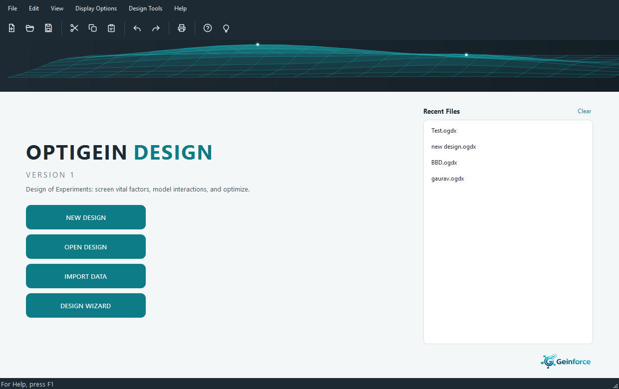
When OptiGein Design opens, it offers you the four things people usually want first: start a new design, open a design you saved earlier, import data you already have, or let the Design Wizard ask a few questions and pick a design for you. Files you worked on recently are listed so you can jump straight back in.
Light and dark
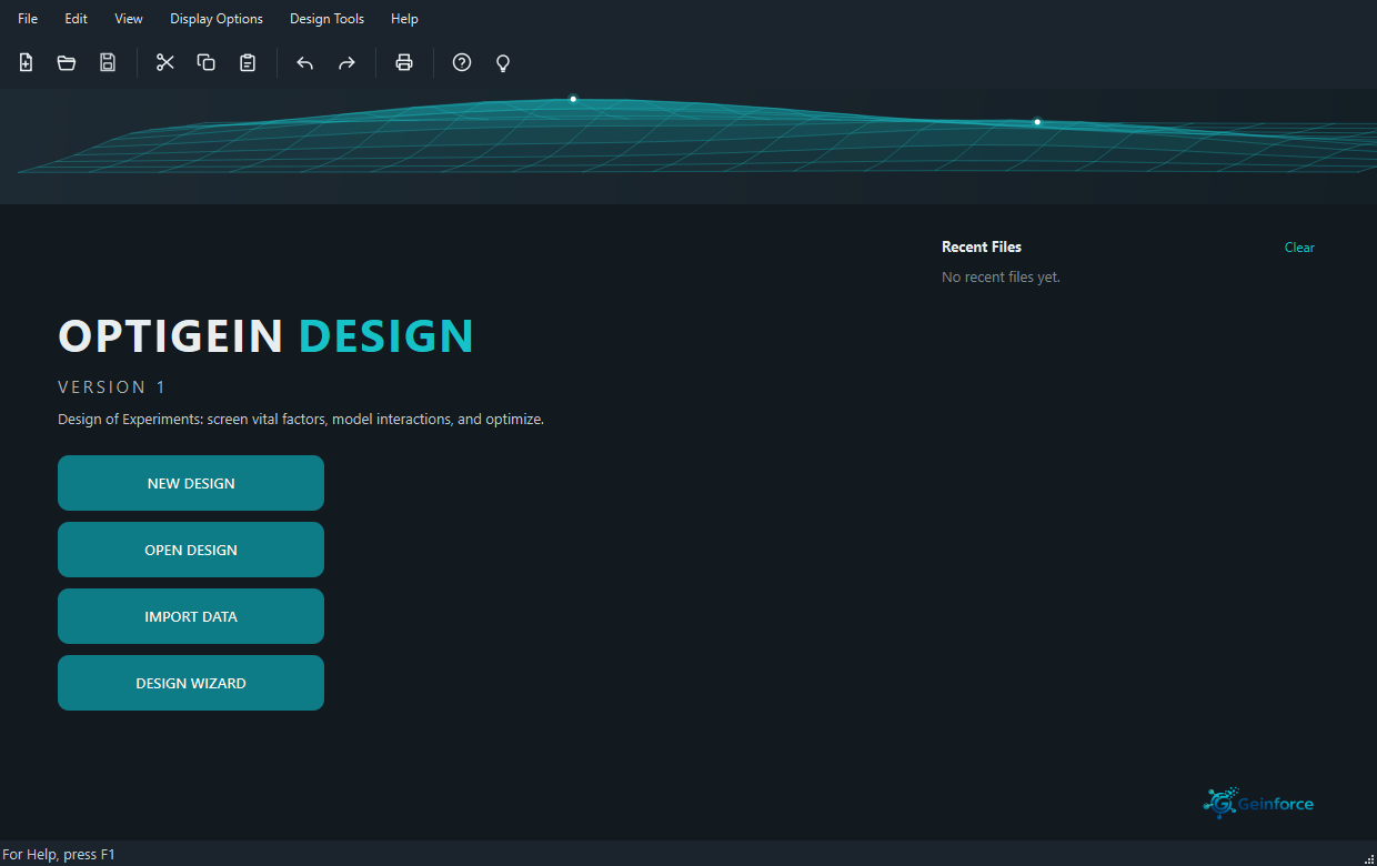
OptiGein Design follows the appearance setting of your operating system. If the computer is set to dark mode, the whole application, including its dialogs, message boxes and tooltips, uses a dark version of the same teal and slate colours. Change the setting in the operating system and the application follows straight away, without a restart. There is nothing to configure inside OptiGein Design itself.
Choosing a design
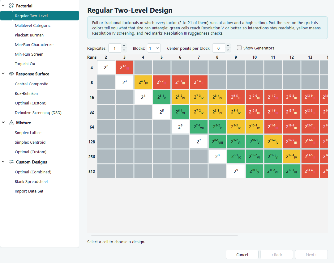
The New Design screen lists every design the software can build, grouped into four families. Select one on the left and the panel on the right explains what it is for and what it costs in runs. Nothing is built until you press Finish, so you can browse freely.
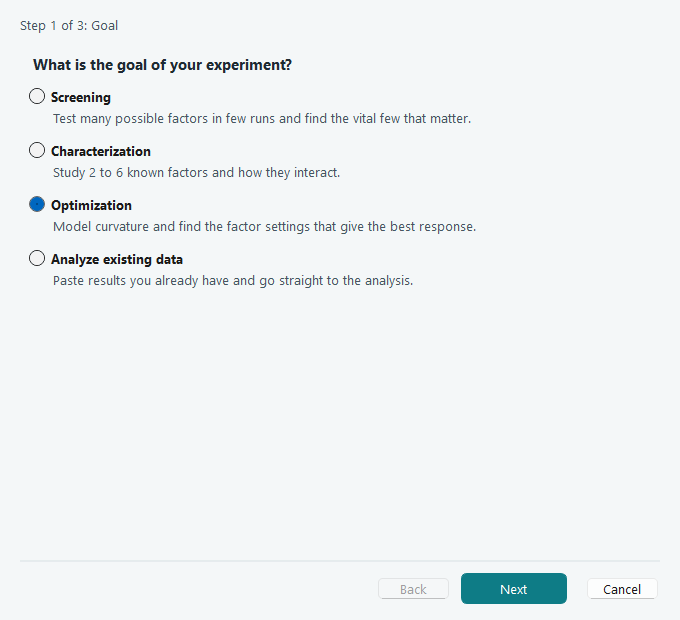
If you would rather answer questions than choose from a list, open the Design Wizard from the Design Tools menu. It asks what stage you are at, how many factors you are studying and how many runs you can afford, then recommends a design and builds it.
The run sheet
Once a design is built, the run sheet appears. Each row is one experiment. The software has already worked out the settings for you; your job is to perform the runs and type the measured responses into the last columns.
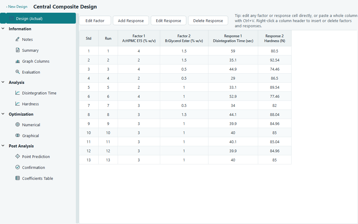
Columns are labelled with the factor letter and the name you gave it, so
A:HPMC E15 (% w/v) is factor A. You can paste a whole column from a spreadsheet with
Ctrl + V, and undo any mistake with Ctrl + Z.
The navigation pane
Everything else lives in the tree on the left. It follows the natural order of an experiment, from the design itself, through analysis, to the optimum.
| Branch | What you do there |
|---|---|
| Design | The run sheet. Enter results, edit factors, add responses. |
| Information | Notes to yourself, a summary of the design, quick plots of the raw columns, and a formal evaluation of the design before you spend money on runs. |
| Analysis | One page per response. Fit a model, read the ANOVA, check the residuals, look at the model graphs. |
| Optimization | Numerical and graphical searches for the settings that satisfy every response at once. |
| Post Analysis | Predict a response at any settings, plan confirmation runs, and read the coefficients table. |
Analysing a response
Click a response under Analysis and you get a strip of tabs that runs left to right in the order you should use them. Configure the model, look at what the data supports, adjust the terms, read the ANOVA, check the diagnostics, then explore the graphs.
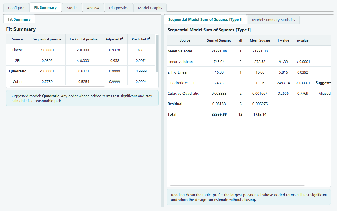
Every table on these screens comes with a short explanation underneath in plain language. If a p-value is small the software says so, and says what that means for the term it belongs to. Full detail is in Fit summary, model and ANOVA.
Seeing the model
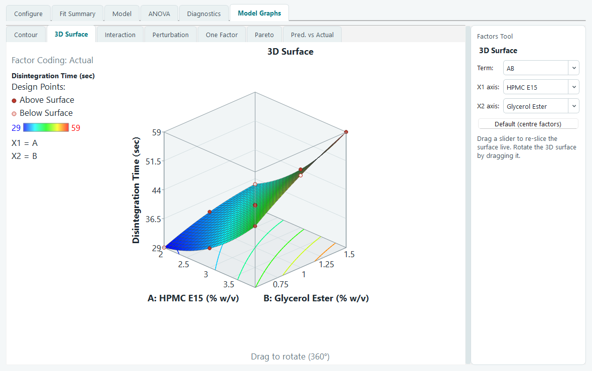
The Model Graphs tab draws the fitted surface. The contour map is the one people put in reports; the 3D surface is the one that makes the shape obvious. Both can be sliced at any setting of the factors you are not plotting.
Finding the optimum
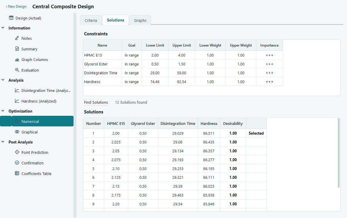
Under Optimization, give each response a goal. The optimizer combines them into a single desirability score and searches the fitted models for the settings that score highest.
What to read next
The fastest way to make all of this concrete is to follow one example from an empty screen to a recommended set of settings.
- Response surface, start to finish, the main tutorial.
- Which design do I need? if you are planning a real experiment now.
- The design workspace for the details of every page in the navigation pane.