Factorial designs
Factorial designs answer the first question of any experiment: out of everything you could change, which factors actually move the result, and by how much. They run each factor at a small number of settings and vary them together, so a handful of runs tells you about many factors at once. This page covers the six designs in the Factorial family and the ideas you need to pick between them.
You reach all six from the New Design screen, listed under Factorial in the catalogue on the left. Select one and the panel on the right explains what it does and how many runs it costs before you build anything. If you are not sure which family you need at all, start with Which design do I need?
Resolution, and why the two-level grid is coloured
When you cannot afford to run every combination of factors, you run a fraction of them. The price of that saving is aliasing: some effects can no longer be told apart, because they were measured on the same set of runs. Resolution is the shorthand for how bad the aliasing is. A higher Roman numeral means cleaner effects. The three you will meet are these.
| Resolution | What stays clear | What is tangled | Use it for |
|---|---|---|---|
| III | Main effects. | A main effect is aliased with two-factor interactions, so a big reading could be the factor or an interaction you cannot separate. | A quick ruggedness or sorting check when you are willing to assume interactions are small. |
| IV | Main effects are clear of every two-factor interaction. | Two-factor interactions are aliased with each other, so you learn that an interaction exists but not which pair caused it. | Screening a long list down to the few factors that matter. |
| V | Main effects and every two-factor interaction are all clear of one another. | Interactions only overlap three-factor and higher terms, which are usually negligible. | Characterising a short list of factors, interactions included. |
OptiGein Design paints this straight onto the two-level grid so you can see the trade at a glance. Green cells reach Resolution V or better, yellow cells are Resolution IV, and red cells are Resolution III. Full factorials sit in the leftmost column with no colour fill, because they alias nothing at all.
Regular Two-Level
This is the workhorse of the family. Every factor, from 2 up to 21 of them, runs at a low and a high setting. You choose the size on a grid whose rows are the number of factors and whose columns are the fraction, from the full factorial on the left through progressively smaller fractions to the right. Each cell shows the run count and its resolution colour, so you are choosing runs and aliasing together in one click.
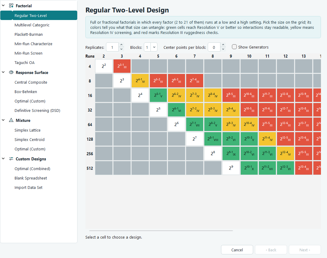
Below the grid are four controls. Replicates repeats the whole design so you can
estimate pure error. Blocks (1, 2, 4 or 8) splits the runs into groups when you
cannot do them all under identical conditions, for example across two days. Center points
per block adds runs at the midpoint of every factor. Show Generators
reveals the defining relation (written I = ...) for a fractional design, which is the
exact statement of what is aliased with what.
Multilevel Categoric
Use this when a factor is a category rather than a dial, or when two settings are not enough. It takes 1 to 12 factors, each with its own list of levels (a supplier, a grade, three temperatures), entered as a comma-separated list. The design then crosses every level of every factor, so each combination becomes exactly one run and the effect of each level can be read straight from the averages in the run sheet.
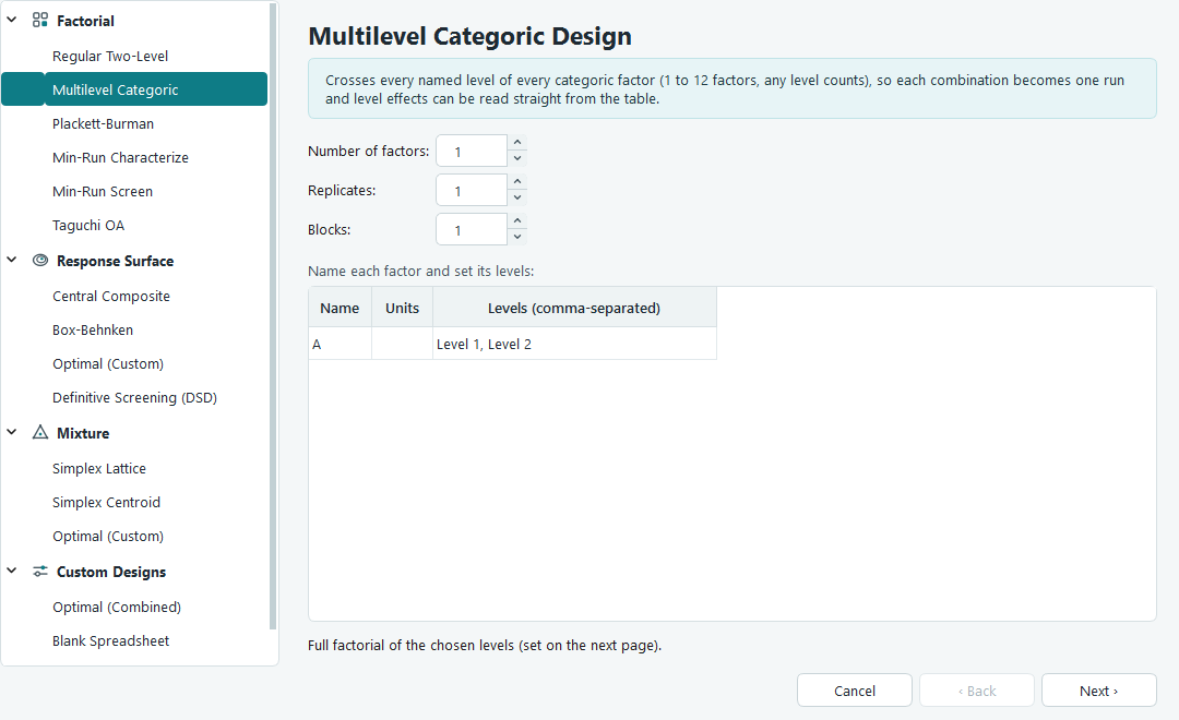
The run count is the product of the level counts, so it grows quickly: three factors at three levels each is already 27 runs before any replication. Replicates and Blocks work as they do for the two-level design. Because this is a full crossing, there is no aliasing to worry about, but the size is the limit rather than the resolution.
Plackett-Burman
When you have many two-level factors and you only want to know which ones matter, Plackett-Burman is the cheapest honest answer. It offers 12, 20 or 24 run sizes and handles up to 23 factors, which is why the number of factors you may enter is capped at one below the run size you pick. Every design is Resolution III.
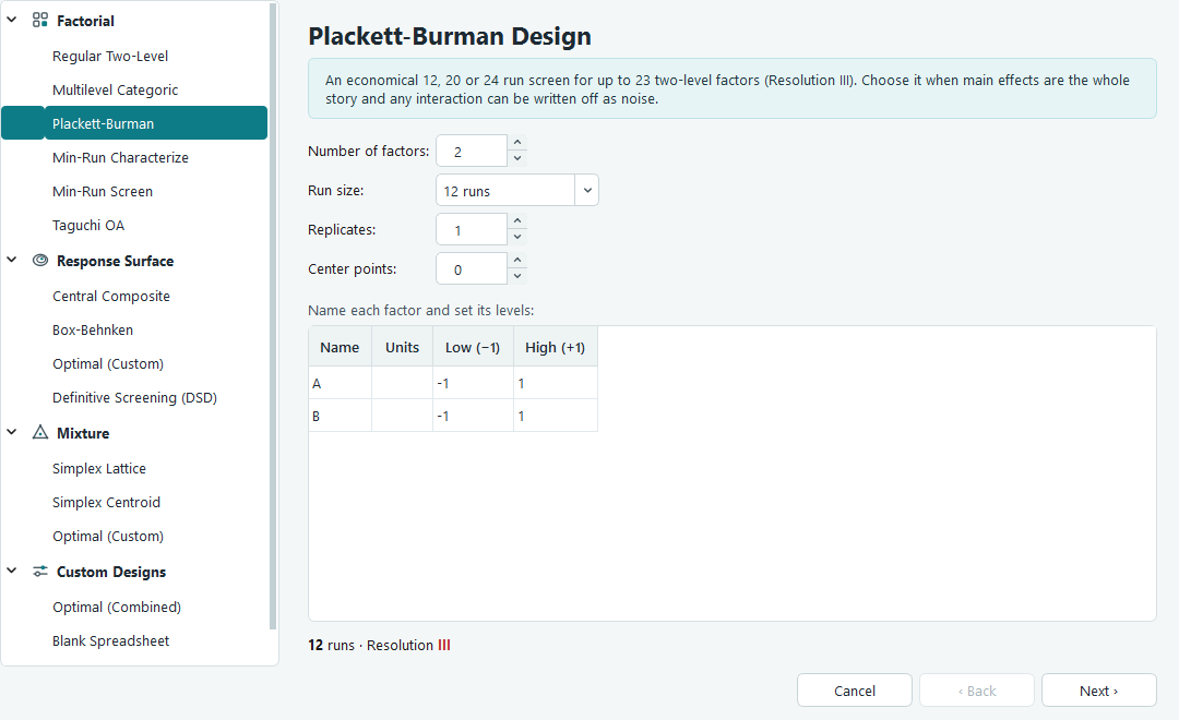
The catch is baked into that Resolution III: main effects are partially aliased with two-factor interactions. You can conclude that a factor looks important, but if an interaction is really driving the response, Plackett-Burman will not tell you. Treat it as a sieve, not a final answer, and follow a promising result with a higher-resolution design on the survivors.
Min-Run Characterize (Resolution V)
A full Resolution V two-level design for many factors can run into hundreds of experiments. This design gives you the same clean reading of every main effect and every two-factor interaction for 6 to 20 factors, at close to the fewest runs the model allows. The software builds it by D-optimal coordinate exchange rather than from a textbook fraction, so it is not tied to a power-of-two size.
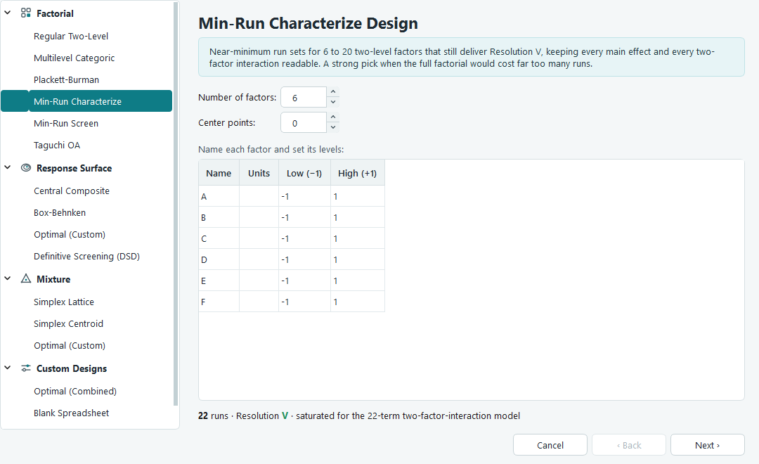
The run count equals the number of terms in the two-factor interaction model, which is
1 + k + k(k-1)/2 for k factors. That makes the plan saturated: at the
minimum it has no spare runs to estimate error. This is why the Center points
control matters here. Adding a few gives you replication for a pure-error estimate and a curvature
check. Choose this design when you need interactions but a full Resolution V fraction is too
expensive.
Min-Run Screen (Resolution IV)
This is the leanest screening design in the family, for 5 to 50 factors at roughly two runs per factor. It is built as a fold-over pair: a compact main-effects half plus its mirror image, which guarantees Resolution IV. Main effects come out clear of every two-factor interaction, while the two-factor interactions overlap one another.
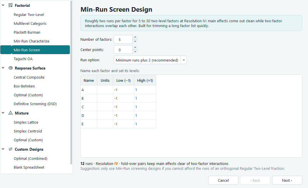
The Run option offers minimum runs, or minimum runs plus 2. The plus-2 choice is the default because it lifts the fit away from saturation and gives a steadier estimate. You can conclude which factors have real main effects and that some interactions are present, but not which interactions. The software itself suggests you prefer an orthogonal Regular Two-Level fraction whenever you can afford one, and only reach for this design when you cannot.
Taguchi OA
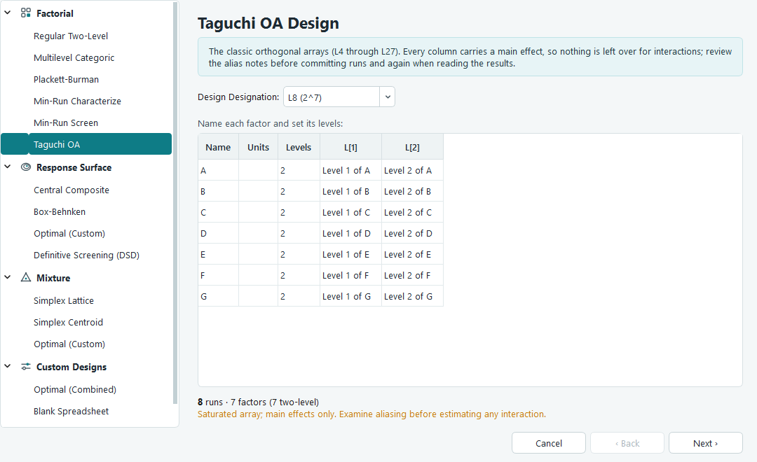
The Taguchi orthogonal arrays are a fixed catalogue of balanced tables: L4, L8, L9, L12, L16, L18, L25 and L27. You pick the designation and the array decides the number of factors and their levels for you; the columns range from two-level (for example L8 holds seven two-level factors) to three and five levels. You only name the factors and their levels. Every column is balanced against every other, so main effects are estimated with equal precision.
Center points, replication and run order
Three settings show up across several of these designs and are worth understanding once.
Center points are runs with every numeric factor set to its midpoint. They do two jobs. Repeated, they give you a pure-error estimate that does not depend on the model being correct. Compared against the average of the factorial runs, they reveal curvature: if the centre sits well off the line between the corners, the response is bending. A two-level design can detect that curvature but cannot map it, so a strong signal is your cue to move up to a response surface design.
Replicates repeat runs so that random measurement scatter can be separated from real effects. More replication sharpens every estimate and is the honest way to earn degrees of freedom for the error term, at the cost of more runs.