Model graphs
The Model Graphs tab draws the fitted model as a picture. The ANOVA tells you a term matters; a model graph shows you what it does. This page explains every graph on the tab, how to read it, and how the Factors Tool on the right decides what you are looking at.
Model Graphs is the last tab in the analysis strip, after Diagnostics. It only has anything to show once you have run Start Analysis, because every curve and surface is evaluated live from the model you fitted. The tab is split into two parts: a row of graph tabs on the left, and the Factors Tool on the right that controls all of them.
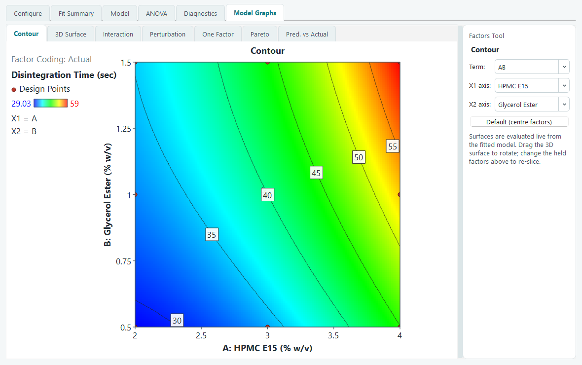
The example used throughout this page is the worked one from the tutorials: a face-centred central composite design with two numeric factors, A: HPMC E15 (2 to 4 % w/v) and B: Glycerol Ester (0.5 to 1.5 % w/v), 13 runs including 5 centre points, analysed for Disintegration Time in seconds.
The Factors Tool: axes and slices
A response surface lives in as many dimensions as you have factors, but a graph is flat. The Factors Tool is how you take a readable two-dimensional slice through it. It changes to match the graph you are on, so it never shows a control that does not apply.
- Which factors go on the axes. For the Contour, 3D Surface and Interaction graphs you pick two: X1 and X2. The Term box is a shortcut that sets both at once from a list of factor pairs (AB and so on). For the One Factor graph you pick a single factor.
- Where the other factors sit. Every factor that is not on an axis gets a slider labelled with its letter and name. The slider runs in coded units from -1 (the low setting) to +1 (the high setting), and the number beside it shows the actual value you are holding it at. Drag a slider and the graph re-slices immediately, so you can watch the surface change as you move a held factor.
The Default (centre factors) button returns every held factor to its centre, which is the natural place to start. Because the example has only two factors and both sit on the axes, it has no held factors and no sliders; the tool becomes busy once you have three or more.
Contour
The contour map is the one people put in reports. It looks straight down on the response surface. X1 runs left to right, X2 runs bottom to top, both in their real units, and the response is shown by colour: cool colours for low values, warm colours for high. Curved iso-lines join points of equal response, each labelled with its value, so you can read a target level straight off the map.
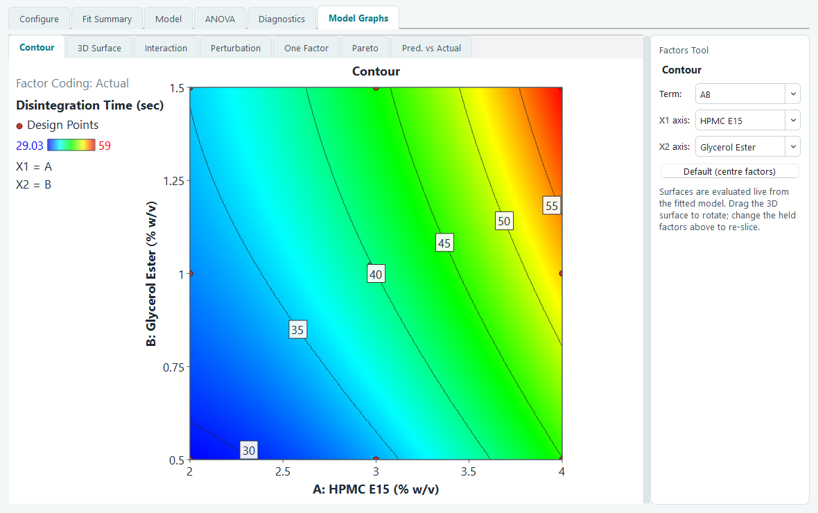
The red dots are your runs, placed at their factor settings. Move the mouse over the map and a small read-out shows the predicted response at the exact spot under the cursor, which is handy for reading a value between the labelled lines. The panel on the left records the response, the colour scale from low to high, and the actual values of any held factors.
3D Surface
The 3D surface shows the same information as the contour map, but lifted into a solid shape, which is the view that makes a peak, a valley or a saddle obvious at a glance. The surface is colour-shaded by height, the floor beneath it carries the same contour lines projected down, and your runs are drawn as dots: filled red where a run sits above the fitted surface, hollow where it sits below.
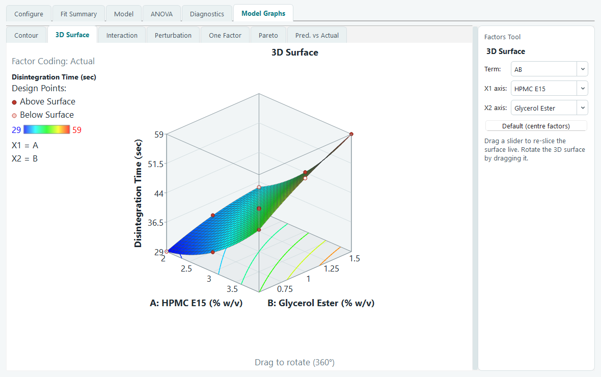
Drag anywhere on the cube to rotate it. Dragging left and right spins it around; dragging up and down tilts it. The cube keeps a fixed size while you rotate, so it never jumps around under the cursor. To set an exact viewpoint instead of hunting for it, right-click the graph and choose Set rotation, then type a horizontal angle and a vertical angle. This is the way to make two surfaces line up for a side-by-side comparison, or to reproduce the same view every time.
Interaction
An interaction graph answers one question: does the effect of one factor depend on the level of another? It plots the predicted response against X1 as a line, drawn twice, once with X2 held at its low setting and once with X2 held high. If the two lines are parallel, the factors act independently. If they fan apart or cross, there is an interaction, and the further from parallel they are, the stronger it is.
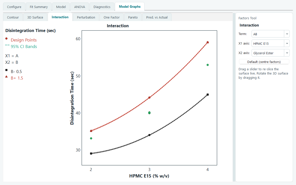
Each line carries a dashed 95% confidence band above and below it. The band is the range the true mean response is expected to lie in, so where a band is wide the prediction is less certain, and where two bands overlap you cannot claim the two levels really differ at that point. Observed runs that lie on the current slice are plotted too, coloured by which level of the second factor they belong to, so you can see the data behind the lines.
Perturbation
The perturbation graph puts every factor on one plot so you can compare their influence at a single point. Starting from a reference point, it moves one factor at a time away from that point and draws how the response changes, giving one curve per factor. The horizontal axis is the coded deviation from the reference, so all factors share the same scale and are directly comparable.
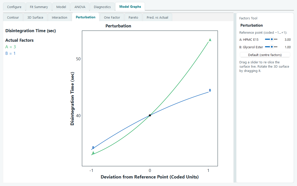
Read it by slope. A steep curve marks a factor the response is sensitive to; a flat curve marks one that barely moves it near this point. A curved rather than straight line signals curvature in that factor. The reference point is set by the sliders in the Factors Tool, which here are labelled as the reference rather than as held factors, so you can ask the same question at the centre, at a corner, or anywhere else worth checking. The black dot is the reference itself, where every curve meets.
One Factor
The One Factor graph is the simplest of the set: the predicted response against a single factor, with the other factors held wherever the sliders leave them. It is the right graph for a factor that the ANOVA showed has no meaningful interactions, because then this single line tells its whole story.
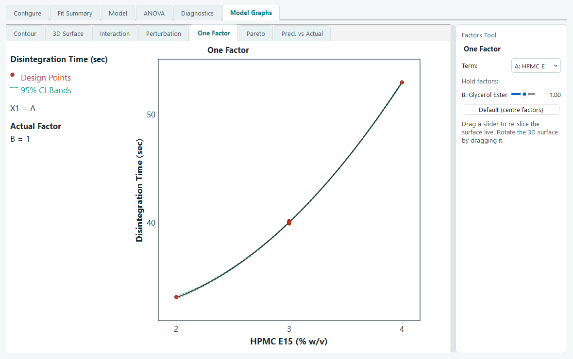
As on the interaction graph, the dashed curves are the 95% confidence band around the fitted line, and the red dots are the observed runs that lie on the slice you are showing. If the points hug the line and stay inside the band, the model describes that factor well.
Pareto
The Pareto chart answers one question at a glance: which terms in the model actually matter? Every term is drawn as a bar whose height is the size of its standardized effect (its t-value), sorted from largest to smallest. Orange bars push the response up, blue bars pull it down, and the term name is written along each bar.
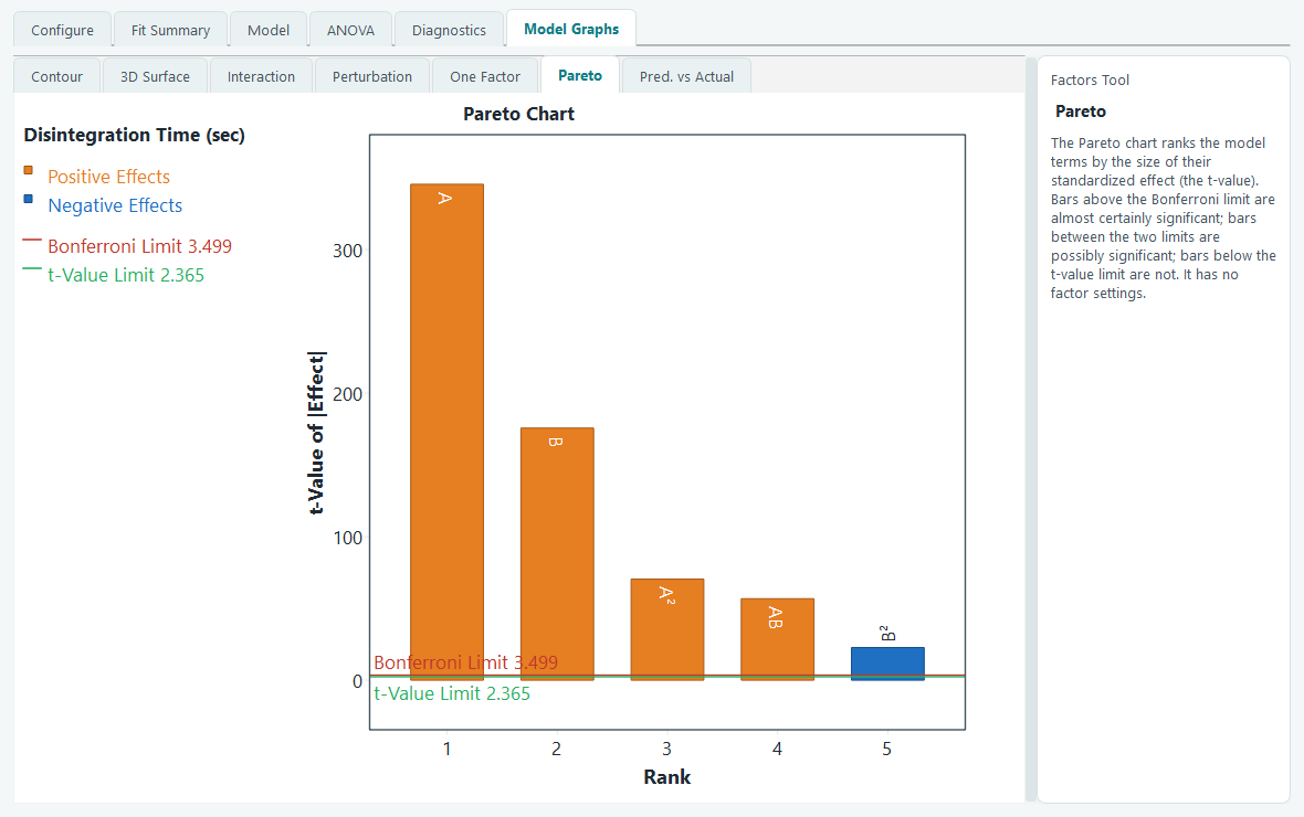
The two horizontal lines are the reference points. A bar that clears the red Bonferroni limit is almost certainly a real effect even after allowing for the number of terms being tested at once. A bar between the two lines is possibly significant, and one below the green t-value limit shows no evidence of an effect. The exact limit values are listed in the left panel, and they match the p-values on the ANOVA page: this chart is the same test drawn as a picture.
The Pareto chart is offered for process designs, where every factor moves independently. Mixture designs do not show it, because the size of a blend component's coefficient depends on how the blend constraint is written into the model, so ranking those bars would mislead.
Predicted versus Actual
The last tab repeats the Predicted versus Actual scatter from the Diagnostics page, so you can keep a check on model quality without leaving the graphs. Each run is a point: its measured response along the bottom, its fitted value up the side. The diagonal line is where a perfect prediction would land.
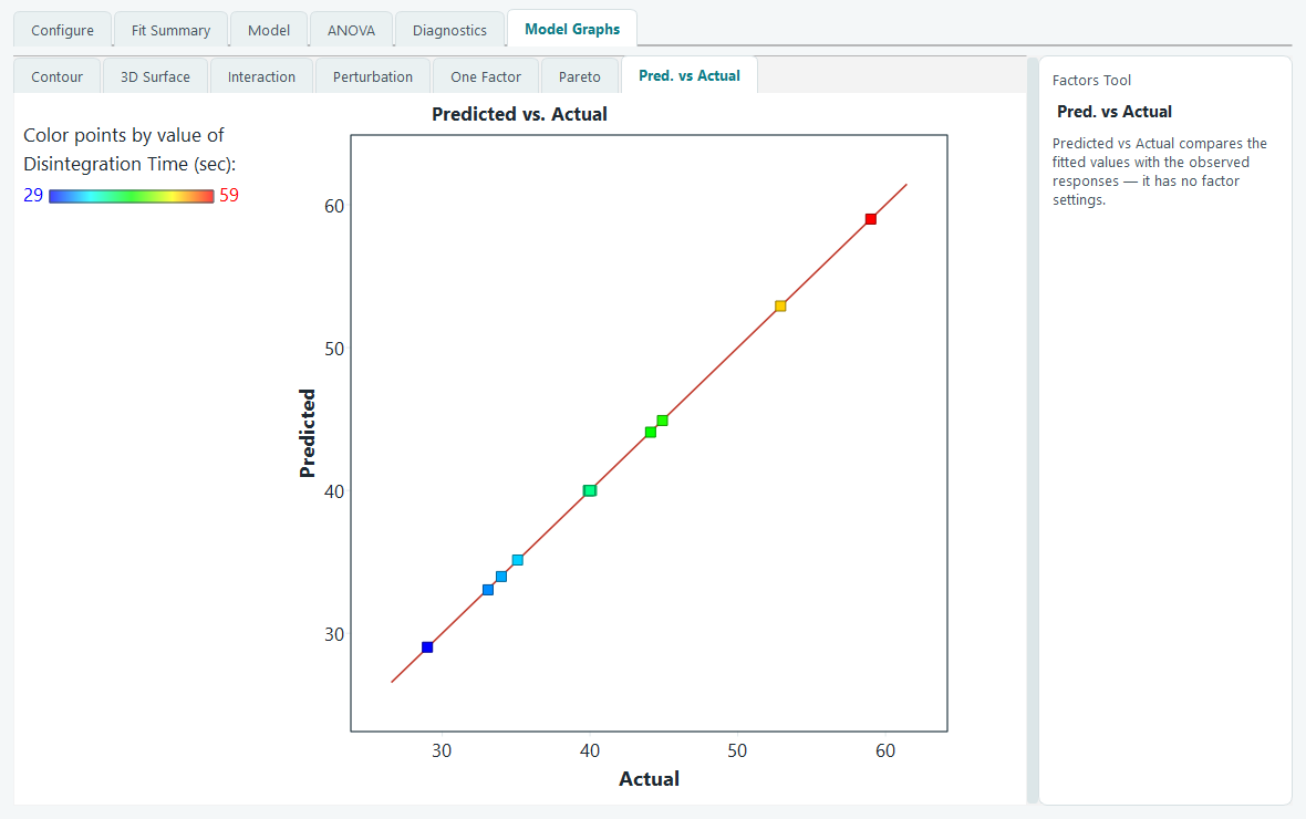
Points that sit tight to the line mean the model is tracking your data. A point that strays far from it is one the model predicts poorly, and is worth a look on the Diagnostics tab to see whether it is an outlier or a sign the model needs another term.
Copying and exporting any graph
Every graph here behaves the same way when you right-click it. You get Copy, which puts the picture on the clipboard ready to paste into a document, and an Export submenu that sends the graph straight into Word or PowerPoint, or saves it as a PNG or JPEG file. On the 3D surface the same menu also carries Set rotation.
With the model understood as a picture, the next step is to ask the software to find the settings that meet every response at once. That is what the optimization pages are for.