Prediction and confirmation
The Post Analysis branch is where you use the models you built. Read off a predicted response at any settings you like, understand how sure the software is about that number, plan how many verification runs to perform, and compare all your response models side by side.
Once you have fitted a model to each response and looked at the diagnostics, the maths is done. Post Analysis turns those models into answers you can act on. It has three pages, and each one answers a different practical question.
| Page | The question it answers |
|---|---|
| Point Prediction | What response should I expect at these exact settings, and how much could it vary? |
| Confirmation | I ran the recipe a few times. Do my results agree with the model? |
| Coefficients Table | How do all my response models compare, term by term? |
Point Prediction
Point Prediction lets you pick any point inside the design space and read off what every response
is expected to be there. In the worked example, a face-centred central composite design on
A:HPMC E15 (% w/v) and B:Glycerol Ester (% w/v), you might ask what
Disintegration Time and Hardness the models predict at 3.2 % HPMC and 0.9 % glycerol ester, a
setting you never actually ran.
The right-hand Factors Tool has one slider per numeric factor. Each slider moves that factor across its range, from its low level to its high level, and the label beside it shows the setting in real units as you drag. The Factors table at the top left echoes the chosen level for each factor next to its low and high values. The Point Prediction table below updates the moment you move a slider.
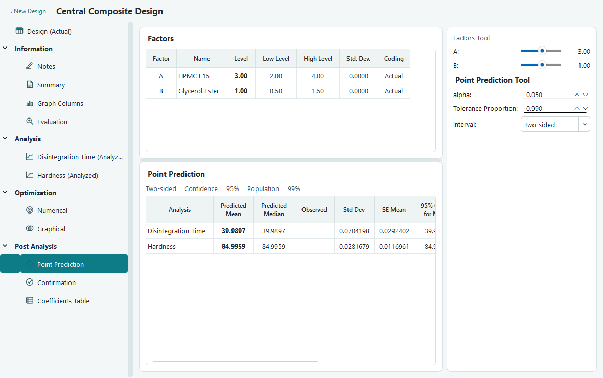
Each row of the Point Prediction table is one response. The columns tell you the prediction and, just as important, how much to trust it.
| Column | What it means |
|---|---|
| Predicted Mean | The model's estimate of the average response at this point. This is the number you would quote. |
| Predicted Median | The predicted middle value. For a response you did not transform, the median equals the mean, so the two columns match. |
| Std Dev | The estimated run to run standard deviation of the response about the model. It comes from the residual mean square and does not change as you move the point. |
| SE Mean | The standard error of the predicted mean. This measures how precisely the model pins down the average at this point. It is smallest near the centre of the design and grows towards the edges and corners. |
| CI low / CI high for Mean | The confidence interval for the average response at this point. |
| TI low / TI high for Pop | The tolerance interval, which brackets a stated proportion of individual future units. |
Notice that Std Dev and SE Mean are different things and people mix them up. Std Dev describes how much a single batch scatters around the true value. SE Mean describes how unsure the model is about where the true average sits, and that depends on where you are in the design: predict near the centre and the software is confident, predict out in a corner where you have little data and it is less confident.
The three controls
Below the sliders, the Point Prediction Tool has three settings that shape the intervals.
| Control | Effect |
|---|---|
| alpha | Sets the confidence level. The level shown is (1 minus alpha). The default 0.05 gives 95 % intervals. Lower it for wider, more cautious intervals. |
| Tolerance Proportion | The fraction of the population the tolerance interval must cover. The default 0.99 asks the interval to contain 99 % of future units. |
| Interval | Two-sided gives a low and a high bound. One-sided is for when you only care about one direction, for example a minimum acceptable hardness. |
The header line above the table restates your choices in words, for instance Two-sided, Confidence = 95 %, Population = 99 %, so the interval columns are never ambiguous.
Confidence interval or tolerance interval?
This is the distinction that trips people up, so it is worth being exact.
| Interval | What it is a statement about |
|---|---|
| Confidence interval for the mean | A range that, with your chosen confidence, contains the true average response at this point. It is narrow, because averages are easier to pin down than individuals. It shrinks as your design gives more information about the mean. |
| Tolerance interval for the population | A range that, with your chosen confidence, contains a stated proportion of individual future units. It is wider, because it must allow for the run to run scatter of single batches, not just the position of the average. |
Confirmation
A model is a prediction until you test it. The Confirmation page helps you plan verification runs at a chosen setting and then check whether what you measured agrees with what the model expected. This closes the loop on the whole experiment.
The layout mirrors Point Prediction. The Factors Tool sliders set the location you want to confirm, shown as Confirmation Location #1 with the factor settings in real units. The difference is the Runs box and the Response data table underneath it.
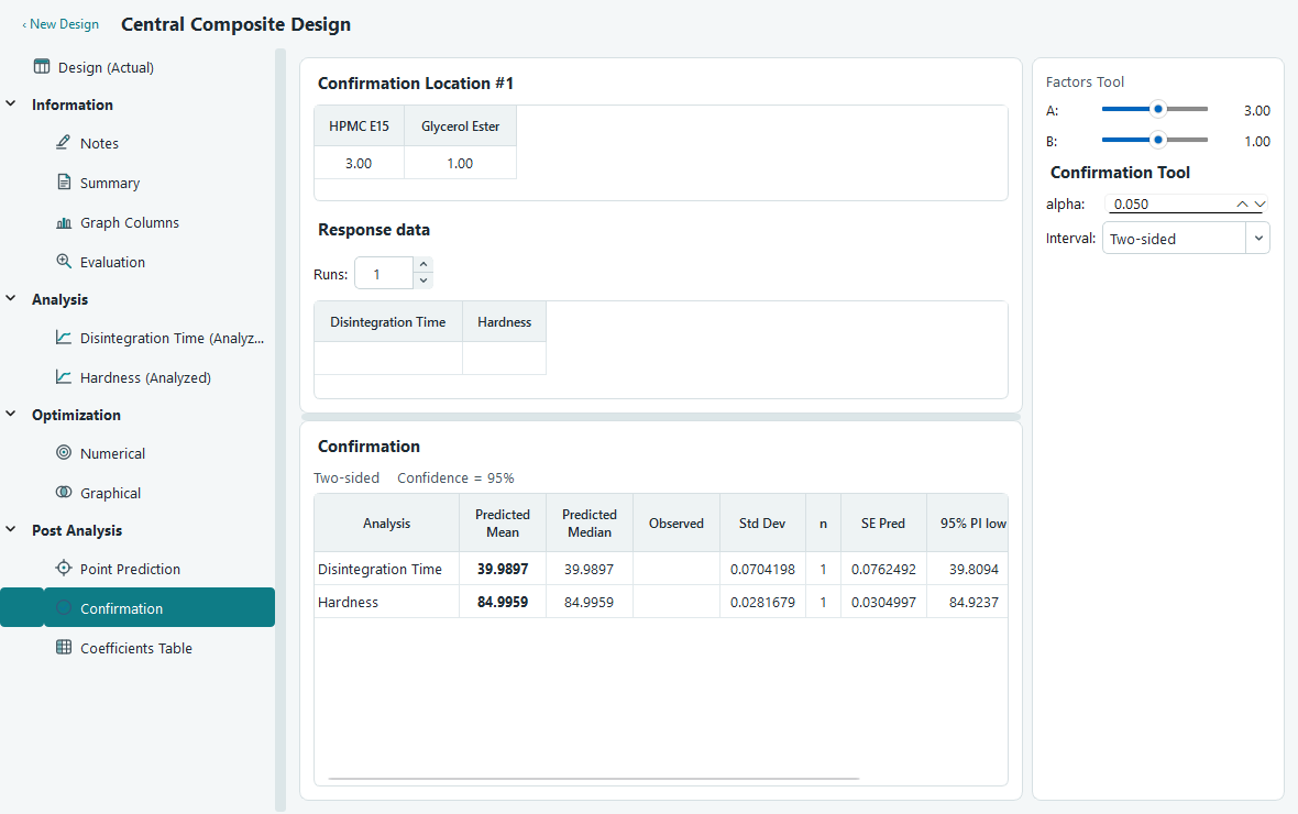
- Move the sliders to the setting you intend to verify. This is usually the optimum you found under the Optimization branch.
- Set Runs to the number of confirmation experiments you plan to perform. This is the n column in the results. Raising n narrows the prediction interval, because the average of several runs is steadier than a single run.
- Perform the runs, then type each measured value into the Response data table. Each analysed response gets its own column.
- Read the Data Mean against the prediction interval. If the average of your confirmation runs lands inside the interval, your results agree with the model.
The Confirmation table gives the prediction for each response at the chosen point.
| Column | What it means |
|---|---|
| Predicted Mean, Predicted Median, Std Dev | The same predictions as on the Point Prediction page. |
| n | The number of confirmation runs you set. It feeds directly into the interval. |
| SE Pred | The standard error of the mean of n future runs. It blends the run to run scatter with the model's own uncertainty, so it is larger than SE Mean and shrinks as you plan more runs. |
| PI low / PI high | The prediction interval. The average of n future runs at this point is expected to fall in this range. |
| Data Mean | The average of the values you typed into the Response data table. This is your evidence. |
If the Data Mean sits comfortably inside the prediction interval, the model has passed its test at that point. If it lands outside, something has drifted since you ran the design, or the model is missing an effect, and it is worth investigating before you rely on the settings.
The alpha and Interval controls behave as they do on the Point Prediction page. There is no population proportion here, because a prediction interval is about the average of your runs rather than a proportion of the population.
Coefficients Table
The Coefficients Table puts every fitted response model into a single grid so you can compare them at a glance. Each column is a model term, and every response contributes two rows: its coded coefficients and, beneath them, the p-values for those terms.
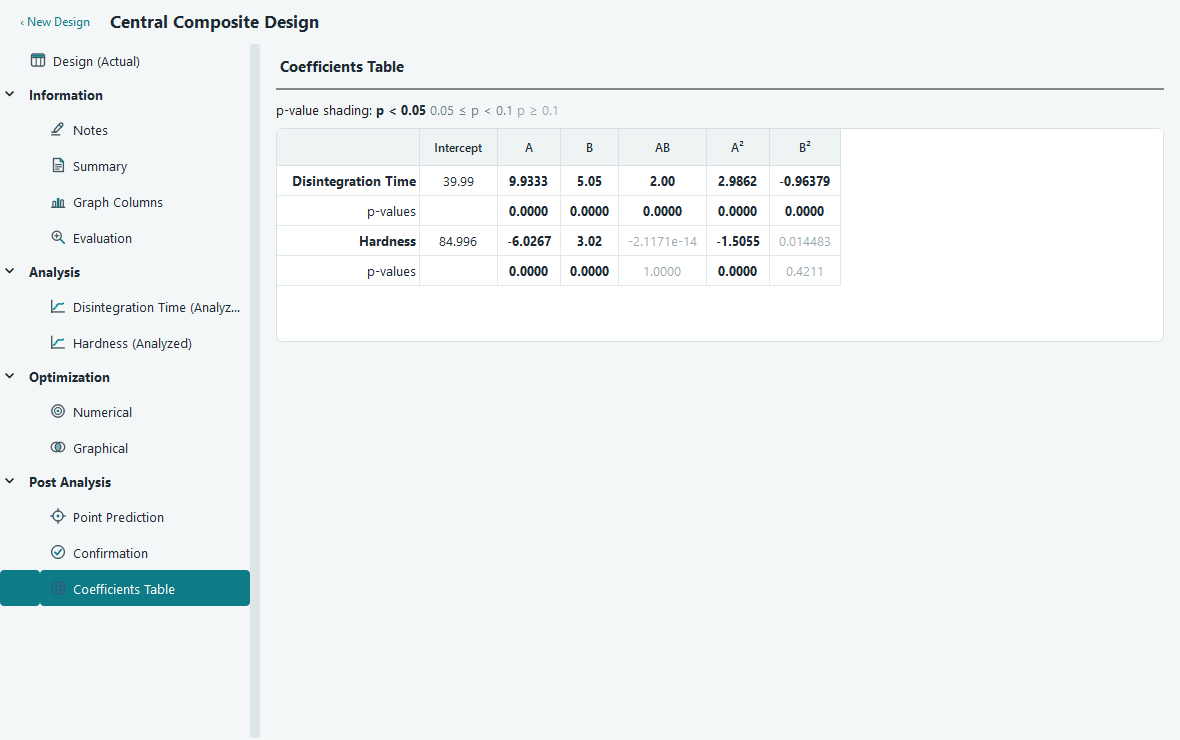
The columns are the pooled list of terms across all your models, ordered from the largest model, so if Disintegration Time carries a curvature term that Hardness does not, that term still gets a column and Hardness simply leaves it blank. A blank cell means the term is not in that response's model.
The p-values are shaded so the important terms stand out without you reading every number. Darker, bold values are significant at p below 0.05. A medium shade marks borderline terms between 0.05 and 0.1. The lightest shade is for terms with p at or above 0.1. The intercept has no p-value, so its cell in the p-value row is left empty.
The coefficients here are in coded units, the same values you see in the coded equation on the Model tab of the Analysis branch. Coded coefficients are directly comparable in size, so a larger coefficient means a stronger effect over the factor's range, which is exactly what makes this table useful for comparison.
Where this fits
Post Analysis is the end of the journey: you built a design, filled in results, fitted and checked models, and searched for the best settings. Here you read predictions at any point, verify them with real runs, and compare your models. The natural next step is to save, print or export what you found.
- Numerical optimization to find the settings you would bring here to confirm.
- Saving, printing and exporting to get these tables into a report. Right-click any table to copy it.
- Glossary for short definitions of confidence, prediction and tolerance intervals.