Response surface, start to finish
One worked example, followed all the way through. You start with an empty screen and finish with a set of factor settings you can hand to the bench, plus a plan to confirm them. Every step explains why you are doing it, not just where to click.
The problem is a small tablet formulation. The tablet has to fall apart quickly once it is swallowed, so Disintegration Time should be short. It also has to survive being packed and handled, so Hardness has to stay above a floor. Those two goals pull in opposite directions: the things that make a tablet hard also tend to make it slow to disintegrate. A response surface design is the right tool here because it maps the curved trade-off between the two and lets the optimizer find the compromise.
Two ingredients are in play: A: HPMC E15, studied from 2 to 4 % w/v, and B: Glycerol Ester, studied from 0.5 to 1.5 % w/v.
-
Start a new central composite design.
From the welcome screen choose New Design, then open the Response Surface family and select
Central Composite. The panel on the right explains that this design combines a two level core
with axial runs and centre replicates. On the setup page set Numeric factors to 2, choose
Face-centered (α = 1) for the axial distance, and set Center points to 5. Face centred
means the axial runs sit on the faces of the square rather than outside it, so each factor only
ever takes three settings: its low, its centre and its high. That keeps every run inside the 2
to 4 and 0.5 to 1.5 ranges you can actually make. The live preview reads
13 runs · 4 factorial + 4 axial + 5 center.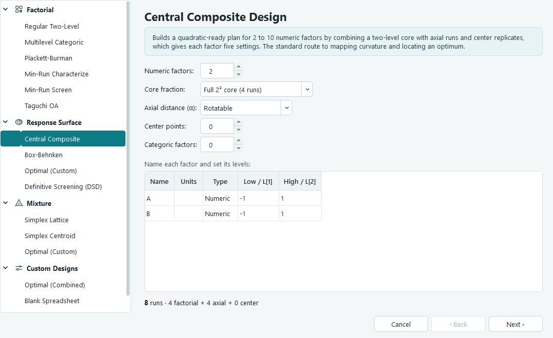
Central Composite setup. The preview line at the bottom updates as you change the options, so you can see the run count before you commit. - Name the factors, set their ranges, add the two responses. In the factor table give factor A the name HPMC E15 with units % w/v, low 2 and high 4. Give factor B the name Glycerol Ester with units % w/v, low 0.5 and high 1.5. The letters A and B stay fixed as the internal names; the text you type is the label that shows up on every table and plot. Move to the next page and set Number of responses to 2, then name them Disintegration Time with units sec and Hardness with units N. Leave Randomize run order ticked. Press Finish to generate the run sheet.
-
Read the run sheet and note the run order.
The design opens on its run sheet under Design in the navigation pane. Each row is one tablet
batch to make and measure. The Std column is the textbook order of the design; the
Run column is the order you should actually work in. The two differ because the run
order is randomised. That matters: if anything drifts during the day, such as humidity or a
warming press, randomising stops that drift from lining up with a factor and masquerading as a
real effect. The response columns on the right are empty and waiting for your measurements.
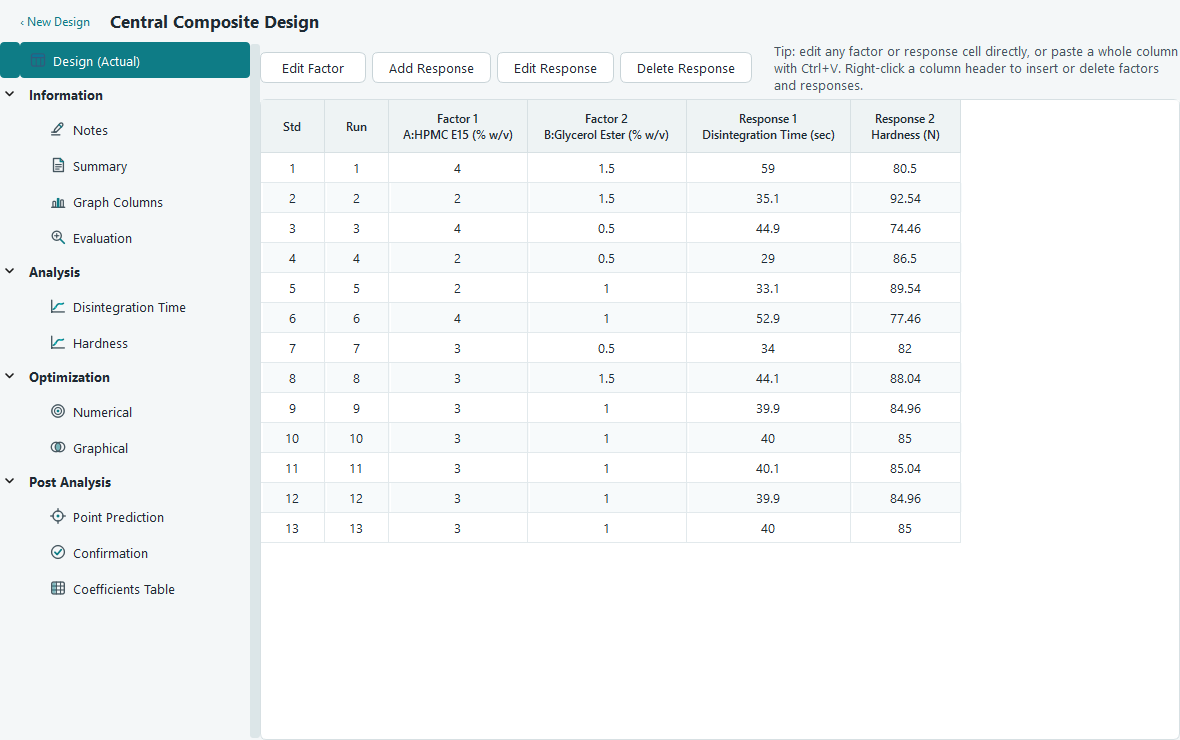
The run sheet. Column headers read like A:HPMC E15 (% w/v)so you can always tell which factor is which. -
Check the design before you spend a day making tablets.
Open Information, then Evaluation. This screen inspects the plan on paper, before any data
exists. Look at the Model Terms table: the power column tells you the design can estimate each
term with even precision, and low variance inflation means the terms are not tangled up with each
other. The Leverage and Degrees of Freedom panels confirm the centre points give you enough pure
error to test lack of fit later. If something here looked wrong, this is the cheap moment to fix
it, by adding runs or centre points, rather than after the experiment.
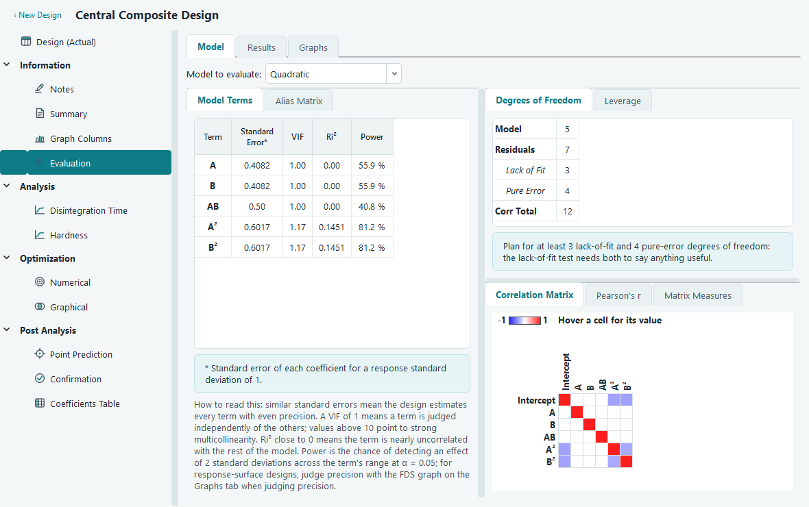
Design evaluation. Green through red shading on the correlation grid flags any pair of terms that overlap. - Perform the runs and enter the results. Make each batch in the Run order shown, measure its disintegration time and hardness, and type the numbers into the matching response cells. You can paste a whole column straight from a spreadsheet with Ctrl + V, and undo any slip with Ctrl + Z. The five centre points are deliberately identical recipes; the spread in their results is your honest estimate of pure experimental noise, which the analysis leans on heavily.
-
Open the first response and start the analysis.
Under Analysis in the navigation pane, click Disintegration Time. You land on the Configure tab.
It confirms how many complete data points it found and offers a Transform and a Polynomial order.
The defaults are sensible for a first pass, so press Start Analysis. The software fits the model
and moves you to Fit Summary.
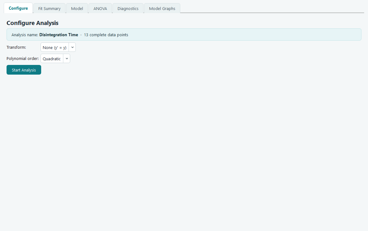
Configure. Changing the order or transform re-arms the Start Analysis button, because the earlier fit is now out of date. -
Read the fit summary and take the suggested model.
Fit Summary compares linear, two factor interaction, quadratic and cubic models side by side and
marks one as Suggested. For a central composite design the suggestion is usually Quadratic,
because that curvature is exactly what the design was built to capture. Two columns guide the
choice: the sequential p-value should be small for the order you keep, meaning its extra terms
genuinely added something, and the lack of fit p-value should not be small, meaning the model
still matches the data. The Adjusted and Predicted R-squared should both be high at the same
time. Accepting the suggestion means leaving the order where the software set it.
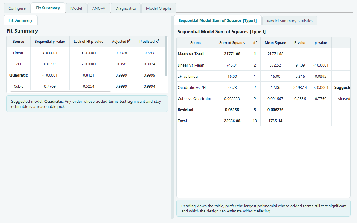
Fit Summary. The suggested row is highlighted, and a short note under the table spells out why in plain language. -
Look at the model terms.
The Model tab lists every candidate term with a status mark. A teal check means the term is in
the fitted model; an amber dot warns that the design cannot estimate that term; the intercept
carries a lock because it is always present. For a two factor quadratic you should see the
intercept, the main effects A and B, the interaction AB, and the squared terms for both factors.
You can right click any term to move it in or out, and the whole analysis re-fits at once, but
for now the suggested set is a good starting point.
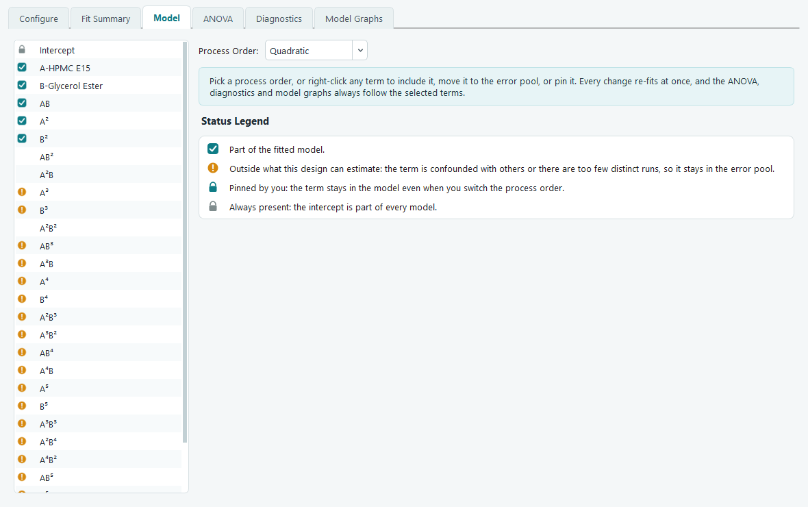
Model terms. Changes here flow straight through to the ANOVA, diagnostics and graphs. -
Read the ANOVA and the equation.
The ANOVA tab tests the model as a whole and each term on its own. Read the top Model row first:
if its p-value is below 0.05 the surface you fitted is unlikely to be an accident of noise. Then
scan the individual rows to see which of A, B, AB and the squared terms carry their weight, again
at p below 0.05. The Lack of Fit row is the reassuring one: you want it not significant, which
says the model misses nothing the pure centre point error can detect. Every table on this tab
comes with a written interpretation underneath, computed from your own numbers. The Actual
Equation writes the fitted model out in real units, so you can predict a disintegration time by
plugging in an HPMC and a glycerol ester level directly.
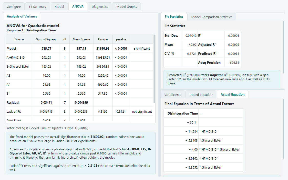
The equation in actual factors. Judge which factor matters most from the coded equation instead, since unit scaling distorts these coefficients. -
Check the diagnostics.
Statistics only mean something if the model's assumptions hold, and the Diagnostics tab is where
you check them. On the normal plot the residuals should fall close to a straight line. On
residuals versus predicted they should scatter in a shapeless band, with no funnel that would
hint the spread grows with the response. On predicted versus actual the points should hug the
diagonal. The influence plots and the Report table flag any single run that is pulling the fit
around more than its share. If everything looks calm, the model is trustworthy.
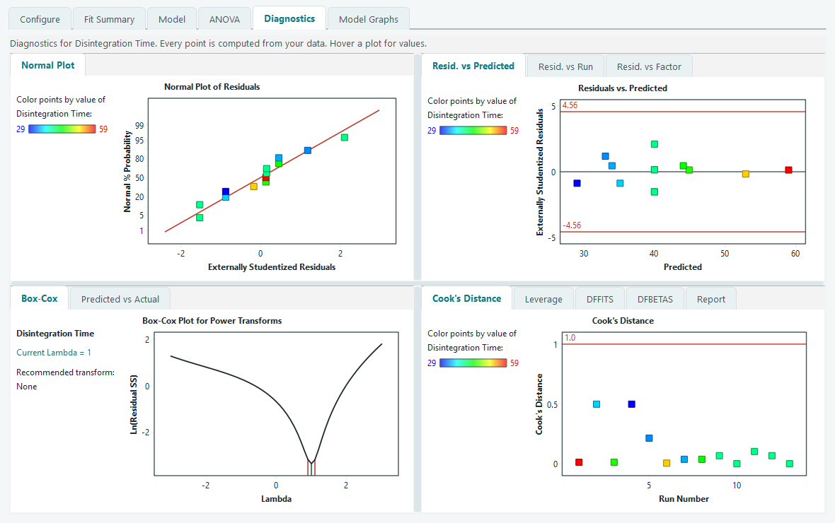
Diagnostics. A pattern here is a signal to try a transform or reconsider the terms, not to ignore it. -
Look at the model graphs.
Now see the surface. The Contour tab draws the map you will put in a report: lines of equal
disintegration time across the HPMC and glycerol ester plane. The 3D Surface makes the shape and
its curvature obvious at a glance. The Interaction plot answers a specific question: if the two
lines are far from parallel, the effect of one factor depends on the level of the other, which is
the AB term earning its place. The Factors Tool on the right lets you slide any factor you are not
plotting and watch the surface re-slice live.
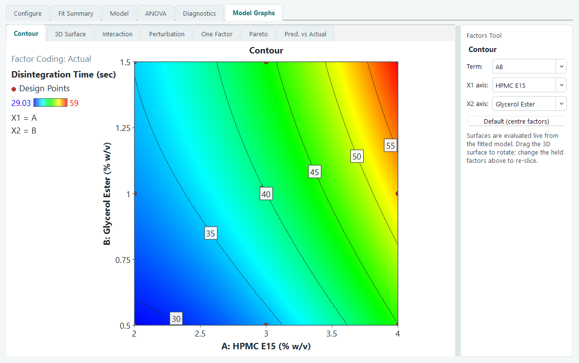
The contour map of Disintegration Time. 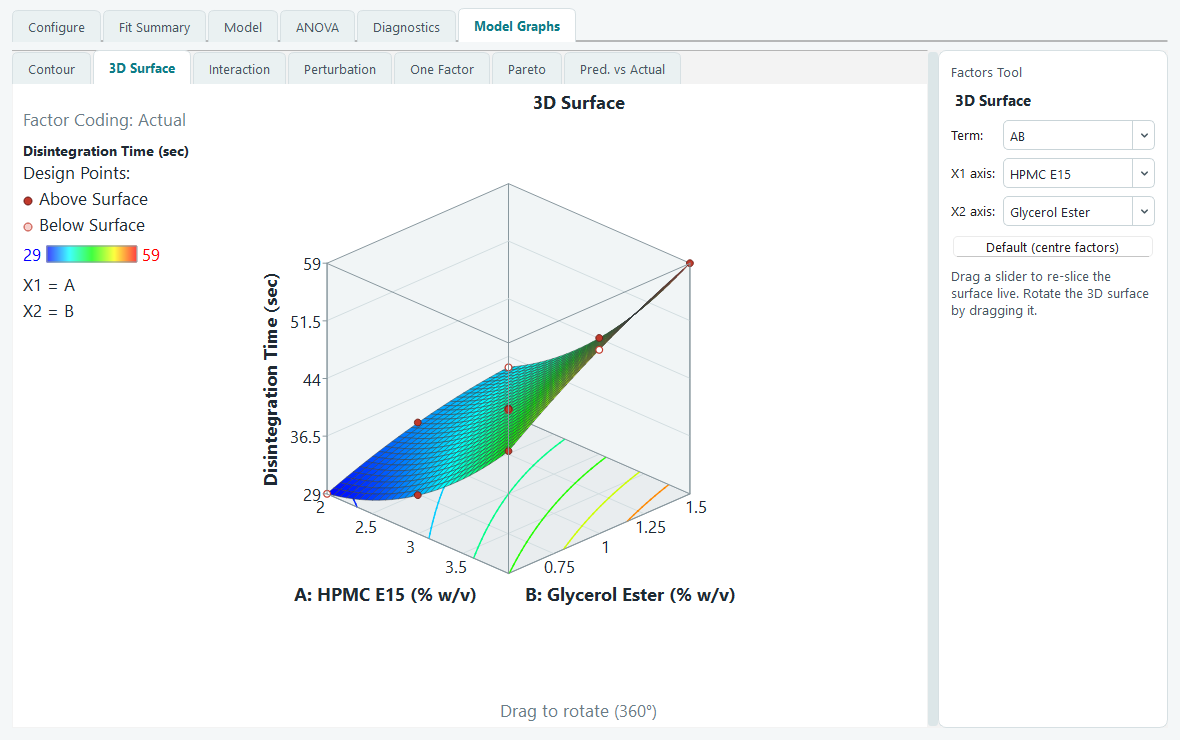
The same fit as a 3D surface, with the design points shown above and below it. 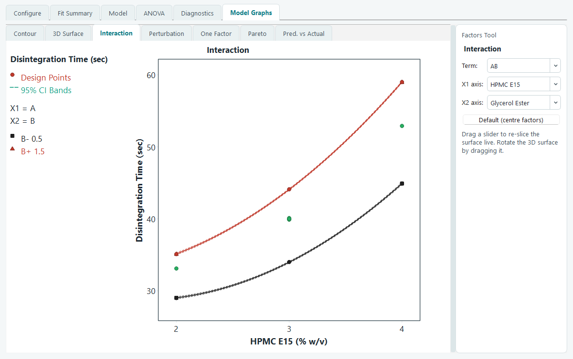
The interaction plot. Non parallel lines mean the two ingredients are not acting independently. - Repeat for the second response. Click Hardness under Analysis and run through the same short loop: Configure, Start Analysis, take the suggested model, glance at the ANOVA, confirm the diagnostics behave. You now have two fitted models over the same design space, one for speed and one for strength. The optimizer needs both before it can look for a compromise.
-
Set goals and run the numerical optimizer.
Open Optimization, then Numerical. The Criteria list holds every factor and every analysed
response. Leave the two factors set to in range, so the search is free to pick any recipe inside
the studied box. Set Disintegration Time to minimize. For Hardness, keep it in range but raise the
lower limit to the softest tablet you can accept, so any recipe below that floor is rejected
outright. Importance and the desirability ramp let you say how hard each goal is pulling. Switch
to Solutions and press Find Solutions. The optimizer combines the goals into a single
desirability score between 0 and 1 and lists the settings that score highest, best first, with
the top row marked Selected.
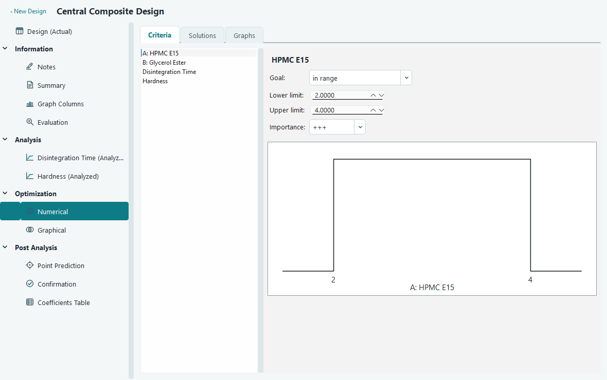
Goals for each response. The ramp on the right shows the desirability shape you are asking for. 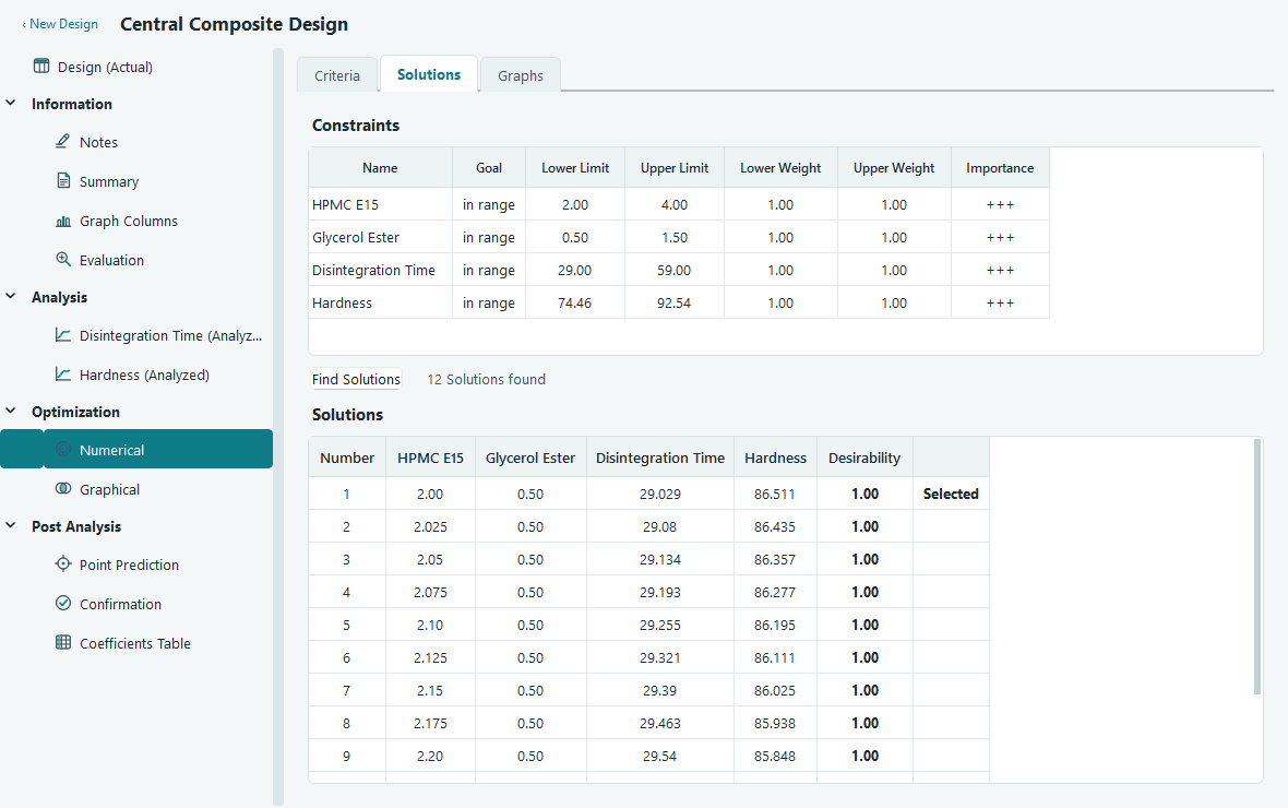
Solutions, best first. Each row is a recipe you could actually make, with its predicted responses and overall desirability. -
Look at the overlay plot to see how much room you have.
A single best point can be fragile. Open Graphical optimization, set a lower and upper limit on
each response to match your specification, and read the overlay plot. The yellow region is where
every response stays inside its limits at once. A wide yellow patch means you have comfortable
room to move if a batch drifts; a thin sliver means the recipe is delicate and worth extra
control. Pick a working point near the middle of the yellow, not on its edge.
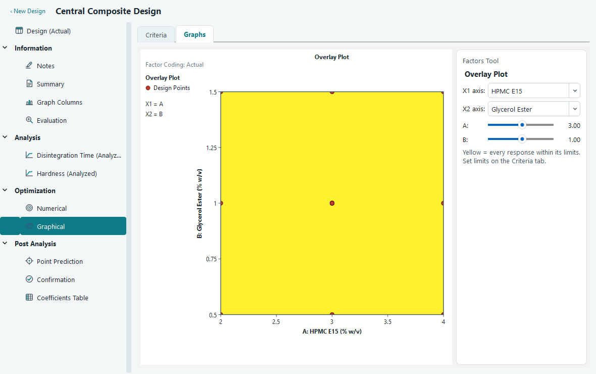
The overlay plot. Yellow is the sweet spot where speed and strength are both acceptable. -
Predict at the chosen settings, then plan confirmation runs.
Under Post Analysis, open Point Prediction. Slide the factors to your chosen HPMC and glycerol
ester levels and read the predicted mean for each response, along with its confidence interval
for the mean and a tolerance interval for the population. The interval, not just the point, is
what you promise. Finally open Confirmation, make a few tablets at exactly those settings, and
type their measured results in. The screen compares your batch mean against the model's
prediction interval. If it lands inside, the model held up and you are done. If it falls outside,
the surface needs another look before you trust it in production.
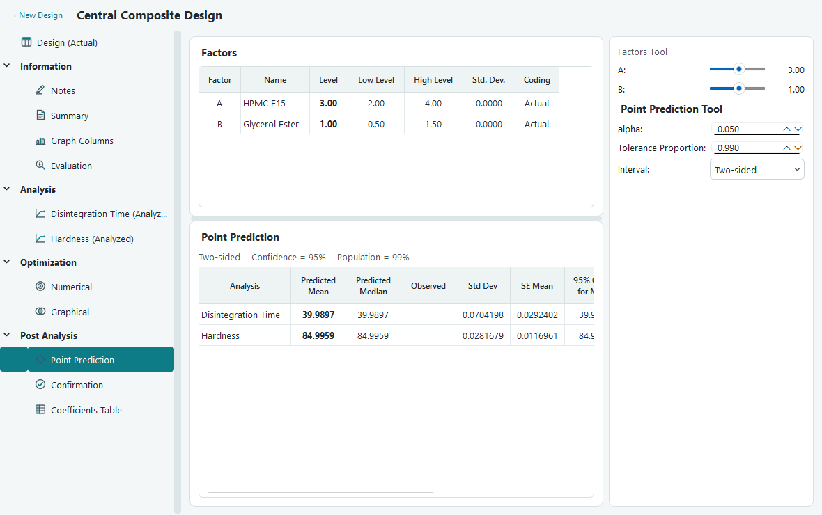
Point prediction at the chosen recipe, with intervals around each mean. 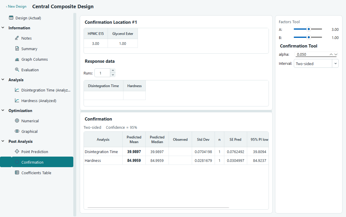
Confirmation. Enter real runs and see whether their mean sits inside the predicted interval.
What you learned
- A face centred central composite design maps curvature on two factors in only 13 runs, with 5 centre points carrying the pure error estimate.
- Randomised run order protects you from drift during the experiment.
- Fit Summary suggests a model, and the ANOVA, diagnostics and graphs tell you whether to trust it.
- The numerical optimizer turns competing goals into one desirability score, and the overlay plot shows how much room the winning settings leave you.
- Point prediction gives you an interval to promise, and confirmation runs prove the model on the bench.
Where to go deeper
- Fit summary, model and ANOVA for what every statistic on those tables means.
- Diagnostics for reading each residual and influence plot.
- Numerical optimization and graphical optimization for goals, weights and limits in full.
- Prediction and confirmation for the intervals behind the last step.