Home › The Surfaces panel
The Surfaces panel
Every field a finished calculation can draw, and the controls that decide how each one looks.
A surface is an isosurface: the set of points where some field takes one chosen value. The Surfaces tab lists the surfaces that exist for the active result, and gives each one its own controls. Ticking an entry draws it, and the same entries appear under the calculation in the project tree.
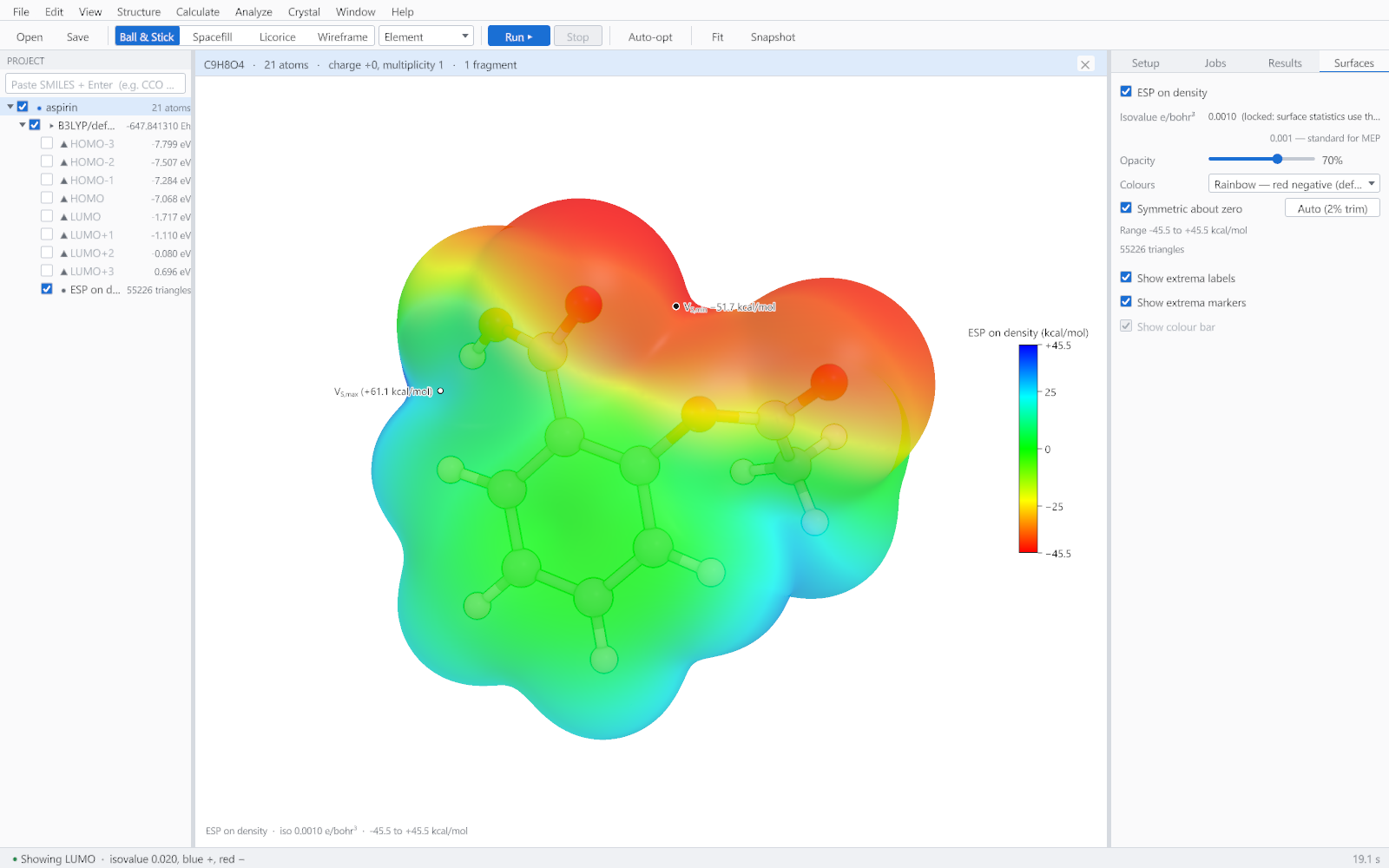
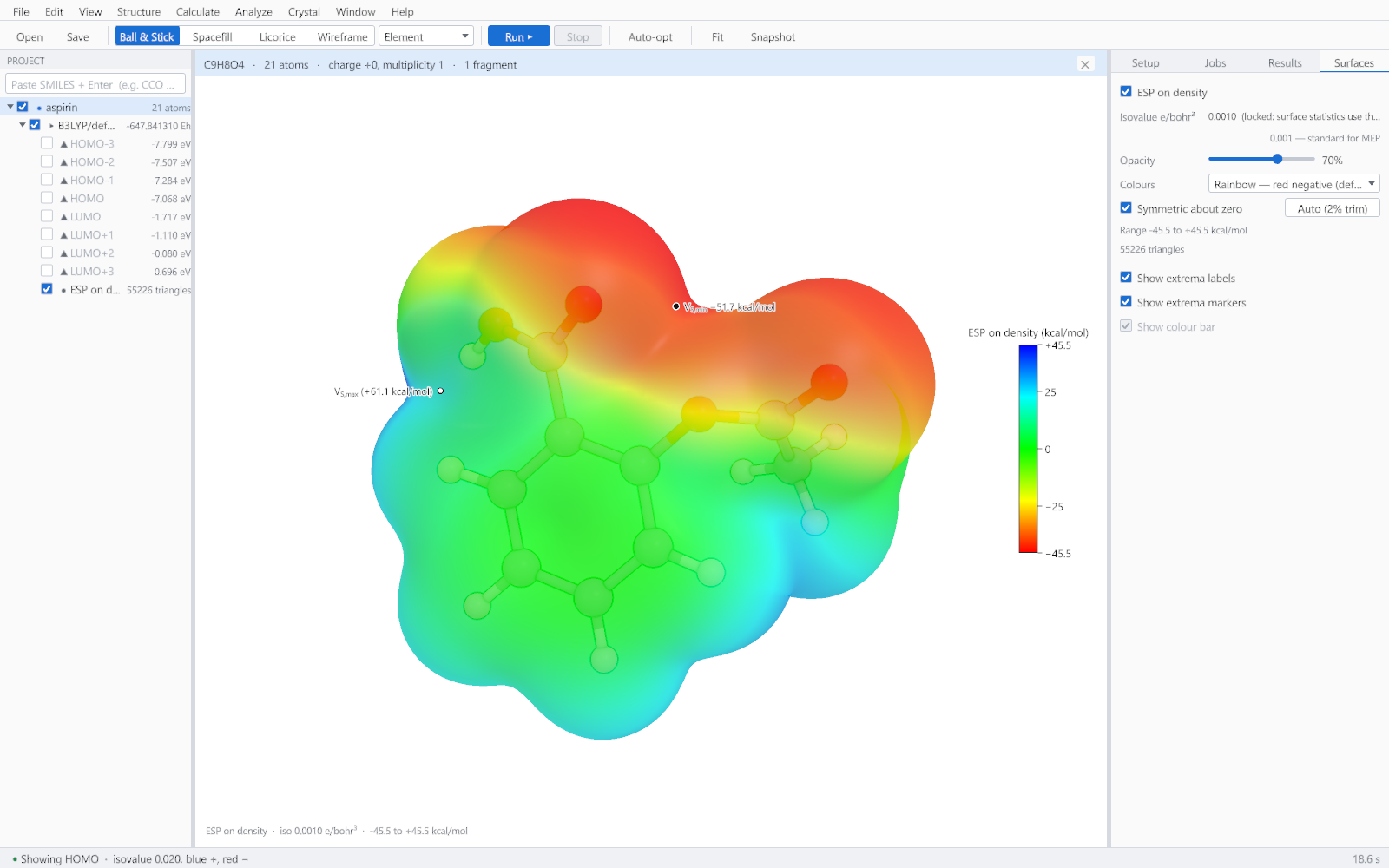
The controls
| Control | What it does |
|---|---|
| Isovalue | The value of the field at which the surface is drawn. For a density surface the unit is electrons per cubic bohr; for an orbital it is the amplitude of the wavefunction. |
| Opacity | How much of the molecule shows through. Around seventy per cent lets the skeleton be seen inside a mapped surface, which is usually what a reader needs. |
| Colours | The colour scale for a mapped surface. The default puts red at negative potential and blue at positive, which is the convention in the literature. |
| Symmetric about zero | Forces the scale to run from minus a value to plus the same value, so that green always means zero. Leave this on when comparing two molecules, since otherwise each gets its own range and the colours mean different things in each picture. |
| Auto | Sets the range from the data, trimming the extreme two per cent so that a single sharp maximum does not flatten the rest of the surface to one colour. |
| Show extrema labels and markers | The most positive and most negative points on the surface, marked and labelled with their values. |
| Show colour bar | The scale beside the picture. It cannot be switched off while a colour-mapped surface is visible, because a mapped surface without its scale is not interpretable. |
Which fields are available
| Field | Available when | Page |
|---|---|---|
| Electron density | Any finished calculation | Density and derived fields |
| Electrostatic potential on the density surface | Any finished calculation | Electrostatic potential surfaces |
| Molecular orbitals | Orbital cubes were requested, or on demand from the level diagram | Orbital surfaces |
| Spin density | An unrestricted calculation, meaning any multiplicity above one | Density and derived fields |
| Laplacian of the density | Any finished calculation | Density and derived fields |
| Average local ionisation energy | Any finished calculation | Density and derived fields |
| Fukui functions | Fukui functions were requested in the setup | Charges and reactivity |
A surface that was not computed during the job can still be produced afterwards: the wavefunction is saved with the result, and the field is evaluated from it on a worker thread while the window stays responsive.
How a surface is built
- The field is evaluated on a three-dimensional grid around the molecule.
- The isosurface is extracted by marching cubes, with the ambiguous cases resolved so that the surface never develops holes or spurious bridges.
- The mesh is smoothed and its normals are taken from the field gradient, which is what makes a lobe look like a smooth object rather than a faceted one.
- For a mapped surface, the mapped quantity is evaluated at every vertex of the finished mesh.